
tf
Related Doc:
package api

Method for combining sparse embeddings.
Method for combining sparse embeddings.
Constant padding mode.
Constant padding mode.
The op pads input with zeros according to the paddings you specify. paddings is an integer tensor with shape
[n, 2], where n is the rank of input. For each dimension D of input, paddings(D, 0) indicates how many
zeros to add before the contents of input in that dimension, and paddings(D, 1) indicates how many zeros to
add after the contents of input in that dimension.
The padded size of each dimension D of the output is equal to
paddings(D, 0) + input.shape(D) + paddings(D, 1).
For example:
// 'input' = [[1, 2, 3], [4, 5, 6]]
// 'paddings' = [[1, 1], [2, 2]]
tf.pad(input, paddings, tf.ConstantPadding(0)) ==>
  [[0, 0, 0, 0, 0, 0, 0],
   [0, 0, 1, 2, 3, 0, 0],
   [0, 0, 4, 5, 6, 0, 0],
   [0, 0, 0, 0, 0, 0, 0]]
Padding mode.
Padding mode.
Partitioning strategy for the embeddings map.
Partitioning strategy for the embeddings map.
Ids are assigned to partitions in a contiguous manner.
Ids are assigned to partitions in a contiguous manner. In this case, 13 ids are split across 5 partitions as:
1, 2], [3, 4, 5], [6, 7, 8], [9, 10], [11, 12.
Combines sparse embeddings by using a weighted sum divided by the total weight.
Combines sparse embeddings by using a weighted sum divided by the total weight.
Each id is assigned to partition p = id % parameters.numPartitions.
Each id is assigned to partition p = id % parameters.numPartitions. For instance, 13 ids are split across 5
partitions as: 5, 10], [1, 6, 11], [2, 7, 12], [3, 8], [4, 9.
Reflective padding mode.
Reflective padding mode.
The op pads input with mirrored values according to the paddings you specify. paddings is an integer tensor
with shape [n, 2], where n is the rank of input. For each dimension D of input, paddings(D, 0)
indicates how many values to add before the contents of input in that dimension, and paddings(D, 1) indicates
how many values to add after the contents of input in that dimension. Both paddings(D, 0) and paddings(D, 1)
must be no greater than input.shape(D) - 1.
The padded size of each dimension D of the output is equal to
paddings(D, 0) + input.shape(D) + paddings(D, 1).
For example:
// 'input' = [[1, 2, 3], [4, 5, 6]]
// 'paddings' = [[1, 1], [2, 2]]
tf.pad(input, paddings, tf.ReflectivePadding) ==>
  [[6, 5, 4, 5, 6, 5, 4],
   [3, 2, 1, 2, 3, 2, 1],
   [6, 5, 4, 5, 6, 5, 4],
   [3, 2, 1, 2, 3, 2, 1]]
Combines sparse embeddings by using a weighted sum.
Combines sparse embeddings by using a weighted sum.
Combines sparse embeddings by using a weighted sum divided by the square root of the sum of the squares of the weights.
Combines sparse embeddings by using a weighted sum divided by the square root of the sum of the squares of the weights.
Symmetric padding mode.
Symmetric padding mode.
The op pads input with mirrored values according to the paddings you specify. paddings is an integer tensor
with shape [n, 2], where n is the rank of input. For each dimension D of input, paddings(D, 0)
indicates how many values to add before the contents of input in that dimension, and paddings(D, 1) indicates
how many values to add after the contents of input in that dimension. Both paddings(D, 0) and paddings(D, 1)
must be no greater than input.shape(D).
The padded size of each dimension D of the output is equal to
paddings(D, 0) + input.shape(D) + paddings(D, 1).
For example:
// 'input' = [[1, 2, 3], [4, 5, 6]]
// 'paddings' = [[1, 1], [2, 2]]
tf.pad(input, paddings, tf.SymmetricPadding) ==>
  [[2, 1, 1, 2, 3, 3, 2],
   [2, 1, 1, 2, 3, 3, 2],
   [5, 4, 4, 5, 6, 6, 5],
   [5, 4, 4, 5, 6, 6, 5]]
The abs op computes the absolute value of a tensor.
The abs op computes the absolute value of a tensor.
Given a tensor x of real numbers, the op returns a tensor containing the absolute value of each element in
x. For example, if x is an input element and y is an output element, the op computes y = |x|.
Given a tensor x of complex numbers, the op returns a tensor of type FLOAT32 or FLOAT64 that is the
magnitude value of each element in x. All elements in x must be complex numbers of the form a + bj. The
magnitude is computed as \sqrt{a2 + b2}. For example:
// Tensor 'x' is [[-2.25 + 4.75j], [-3.25 + 5.75j]]
abs(x) ==> [5.25594902, 6.60492229]
Input tensor that must be one of the following types: HALF, FLOAT32, FLOAT64, INT32, INT64,
COMPLEX64, or COMPLEX128.
Name for the created op.
Created op output.
The accumulateN op adds all input tensors element-wise.
The accumulateN op adds all input tensors element-wise.
This op performs the same operation as the addN op, but it does not wait for all of its inputs to be ready
before beginning to sum. This can save memory if the inputs become available at different times, since the
minimum temporary storage is proportional to the output size, rather than the inputs size.
Input tensors.
Shape of the elements of inputs (in case it's not known statically and needs to be retained).
Created op name.
Created op output.
InvalidArgumentException If any of the inputs has a different data type and/or shape than the rest.
The acos op computes the inverse cosine of a tensor element-wise.
The acos op computes the inverse cosine of a tensor element-wise. I.e., y = \acos{x}.
Input tensor that must be one of the following types: HALF, FLOAT32, FLOAT64, INT32, INT64,
COMPLEX64, or COMPLEX128.
Name for the created op.
Created op output.
The acosh op computes the inverse hyperbolic cosine of a tensor element-wise.
The acosh op computes the inverse hyperbolic cosine of a tensor element-wise. I.e., y = \acosh{x}.
Input tensor that must be one of the following types: HALF, FLOAT32, FLOAT64, INT32, INT64,
COMPLEX64, or COMPLEX128.
Name for the created op.
Created op output.
The add op adds two tensors element-wise.
The add op adds two tensors element-wise. I.e., z = x + y.
NOTE: This op supports broadcasting. More information about broadcasting can be found [here](http://docs.scipy.org/doc/numpy/user/basics.broadcasting.html).
First input tensor that must be one of the following types: HALF, FLOAT32, FLOAT64, UINT8,
INT8, INT16, INT32, INT64, COMPLEX64, COMPLEX128, or STRING.
Second input tensor that must be one of the following types: HALF, FLOAT32, FLOAT64, UINT8,
INT8, INT16, INT32, INT64, COMPLEX64, COMPLEX128, or STRING.
Name for the created op.
Created op output.
The addBias op adds bias to value.
The addBias op adds bias to value.
The op is (mostly) a special case of add where bias is restricted to be one-dimensional (i.e., has rank
1). Broadcasting is supported and so value may have any number of dimensions. Unlike add, the type of
biasis allowed to differ from that of value value in the case where both types are quantized.
Value tensor.
Bias tensor that must be one-dimensional (i.e., it must have rank 1).
Data format of the input and output tensors. With the default format NWCFormat, the
bias tensor will be added to the last dimension of the value tensor. Alternatively, the
format could be NCWFormat, and the bias tensor would be added to the third-to-last
dimension.
Name for the created op.
Created op output.
The addN op adds all input tensors element-wise.
The addN op adds all input tensors element-wise.
Input tensors.
Created op name.
Created op output.
The all op computes the logical AND of elements across axes of a tensor.
The all op computes the logical AND of elements across axes of a tensor.
Reduces input along the axes given in axes. Unless keepDims is true, the rank of the tensor is reduced
by 1 for each entry in axes. If keepDims is true, the reduced axes are retained with size 1.
If axes is null, then all axes are reduced, and a tensor with a single element is returned.
For example:
// 'x' is [[true, true], [false, false]]
all(x) ==> false
all(x, 0) ==> [false, false]
all(x, 1) ==> [true, false]
Input tensor to reduce.
Integer tensor containing the axes to reduce. If null, then all axes are reduced.
If true, retain the reduced axes.
Name for the created op.
Created op output.
The angle op returns the element-wise complex argument of a tensor.
The angle op returns the element-wise complex argument of a tensor.
Given a numeric tensor input, the op returns a tensor with numbers that are the complex angle of each element
in input. If the numbers in input are of the form a + bj, where *a* is the real part and *b* is the
imaginary part, then the complex angle returned by this operation is of the form atan2(b, a).
For example:
// 'input' is [-2.25 + 4.75j, 3.25 + 5.75j]
angle(input) ==> [2.0132, 1.056]
If input is real-valued, then a tensor containing zeros is returned.
Input tensor.
Name for the created op.
Created op output.
IllegalArgumentException If the provided tensor is not numeric.
The any op computes the logical OR of elements across axes of a tensor.
The any op computes the logical OR of elements across axes of a tensor.
Reduces input along the axes given in axes. Unless keepDims is true, the rank of the tensor is reduced
by 1 for each entry in axes. If keepDims is true, the reduced axes are retained with size 1.
If axes is null, then all axes are reduced, and a tensor with a single element is returned.
For example:
// 'x' is [[true, true], [false, false]]
any(x) ==> true
any(x, 0) ==> [true, true]
any(x, 1) ==> [true, false]
Input tensor to reduce.
Integer tensor containing the axes to reduce. If null, then all axes are reduced.
If true, retain the reduced axes.
Name for the created op.
Created op output.
The approximatelyEqual op computes the truth value of abs(x - y) < tolerance element-wise.
The approximatelyEqual op computes the truth value of abs(x - y) < tolerance element-wise.
NOTE: This op supports broadcasting. More information about broadcasting can be found [here](http://docs.scipy.org/doc/numpy/user/basics.broadcasting.html).
First input tensor.
Second input tensor.
Comparison tolerance value.
Name for the created op.
Created op output.
The argmax op returns the indices with the largest value across axes of a tensor.
The argmax op returns the indices with the largest value across axes of a tensor.
Note that in case of ties the identity of the return value is not guaranteed.
Input tensor.
Integer tensor containing the axes to reduce. If null, then all axes are reduced.
Data type for the output tensor. Must be INT32 or INT64.
Name for the created op.
Created op output.
The argmin op returns the indices with the smallest value across axes of a tensor.
The argmin op returns the indices with the smallest value across axes of a tensor.
Note that in case of ties the identity of the return value is not guaranteed.
Input tensor.
Integer tensor containing the axes to reduce. If null, then all axes are reduced.
Name for the created op.
Created op output.
The asin op computes the inverse sine of a tensor element-wise.
The asin op computes the inverse sine of a tensor element-wise. I.e., y = \asin{x}.
Input tensor that must be one of the following types: HALF, FLOAT32, FLOAT64, INT32, INT64,
COMPLEX64, or COMPLEX128.
Name for the created op.
Created op output.
The asinh op computes the inverse hyperbolic sine of a tensor element-wise.
The asinh op computes the inverse hyperbolic sine of a tensor element-wise. I.e., y = \asinh{x}.
Input tensor that must be one of the following types: HALF, FLOAT32, FLOAT64, INT32, INT64,
COMPLEX64, or COMPLEX128.
Name for the created op.
Created op output.
The assert op asserts that the provided condition is true.
The assert op asserts that the provided condition is true.
If condition evaluates to false, then the op prints all the op outputs in data. summarize determines how
many entries of the tensors to print.
Note that to ensure that assert executes, one usually attaches it as a dependency:
// Ensure maximum element of x is smaller or equal to 1.
val assertOp = tf.assert(tf.lessEqual(tf.max(x), 1.0), Seq(x))
Op.createWith(controlDependencies = Set(assertOp)) {
  ... code using x ...
}
Condition to assert.
Op outputs whose values are printed if condition is false.
Number of tensor entries to print.
Name for the created op.
Created op.
The assertAtMostNTrue op asserts that at most n of the provided predicates can evaluate to true at the
same time.
The assertAtMostNTrue op asserts that at most n of the provided predicates can evaluate to true at the
same time.
Sequence containing scalar boolean tensors, representing the predicates.
Maximum number of predicates allowed to be true.
Optional message to include in the error message, if the assertion fails.
Number of tensor entries to print.
Name for the created op.
Created op.
The assertEqual op asserts that the condition x == y holds element-wise.
The assertEqual op asserts that the condition x == y holds element-wise.
Example usage:
val output = tf.createWith(controlDependencies = Set(tf.assertEqual(x, y)) {
  x.sum()
}
The condition is satisfied if for every pair of (possibly broadcast) elements x(i), y(i), we have
x(i) == y(i). If both x and y are empty, it is trivially satisfied.
First input tensor.
Second input tensor.
Optional message to include in the error message, if the assertion fails.
Op outputs whose values are printed if condition is false.
Number of tensor entries to print.
Name for the created op.
Created op.
The assertGreater op asserts that the condition x > y holds element-wise.
The assertGreater op asserts that the condition x > y holds element-wise.
Example usage:
val output = tf.createWith(controlDependencies = Set(tf.assertGreater(x, y)) {
  x.sum()
}
The condition is satisfied if for every pair of (possibly broadcast) elements x(i), y(i), we have
x(i) > y(i). If both x and y are empty, it is trivially satisfied.
First input tensor.
Second input tensor.
Optional message to include in the error message, if the assertion fails.
Op outputs whose values are printed if condition is false.
Number of tensor entries to print.
Name for the created op.
Created op.
The assertGreaterEqual op asserts that the condition x >= y holds element-wise.
The assertGreaterEqual op asserts that the condition x >= y holds element-wise.
Example usage:
val output = tf.createWith(controlDependencies = Set(tf.assertGreaterEqual(x, y)) {
  x.sum()
}
The condition is satisfied if for every pair of (possibly broadcast) elements x(i), y(i), we have
x(i) >= y(i). If both x and y are empty, it is trivially satisfied.
First input tensor.
Second input tensor.
Optional message to include in the error message, if the assertion fails.
Op outputs whose values are printed if condition is false.
Number of tensor entries to print.
Name for the created op.
Created op.
The assertLess op asserts that the condition x < y holds element-wise.
The assertLess op asserts that the condition x < y holds element-wise.
Example usage:
val output = tf.createWith(controlDependencies = Set(tf.assertLess(x, y)) {
  x.sum()
}
The condition is satisfied if for every pair of (possibly broadcast) elements x(i), y(i), we have
x(i) < y(i). If both x and y are empty, it is trivially satisfied.
First input tensor.
Second input tensor.
Optional message to include in the error message, if the assertion fails.
Op outputs whose values are printed if condition is false.
Number of tensor entries to print.
Name for the created op.
Created op.
The assertLessEqual op asserts that the condition x <= y holds element-wise.
The assertLessEqual op asserts that the condition x <= y holds element-wise.
Example usage:
val output = tf.createWith(controlDependencies = Set(tf.assertLessEqual(x, y)) {
  x.sum()
}
The condition is satisfied if for every pair of (possibly broadcast) elements x(i), y(i), we have
x(i) <= y(i). If both x and y are empty, it is trivially satisfied.
First input tensor.
Second input tensor.
Optional message to include in the error message, if the assertion fails.
Op outputs whose values are printed if condition is false.
Number of tensor entries to print.
Name for the created op.
Created op.
The assertNear op asserts that x and y are close element-wise.
The assertNear op asserts that x and y are close element-wise.
Example usage:
val output = tf.createWith(controlDependencies = Set(tf.assertNear(x, y, relTolerance, absTolerance)) {
  x.sum()
}
The condition is satisfied if for every pair of (possibly broadcast) elements x(i), y(i), we have
tf.abs(x(i) - y(i)) <= absTolerance + relTolerance * tf.abs(y(i)). If both x and y are empty, it is
trivially satisfied.
First input tensor.
Second input tensor.
Comparison relative tolerance value.
Comparison absolute tolerance value.
Optional message to include in the error message, if the assertion fails.
Op outputs whose values are printed if condition is false.
Number of tensor entries to print.
Name for the created op.
Created op.
The assertNegative op asserts that the condition input < 0 holds element-wise.
The assertNegative op asserts that the condition input < 0 holds element-wise.
Example usage:
val output = tf.createWith(controlDependencies = Set(tf.assertNegative(x)) {
  x.sum()
}
If input is an empty tensor, the condition is trivially satisfied.
Input tensor to check.
Optional message to include in the error message, if the assertion fails.
Op outputs whose values are printed if condition is false.
Number of tensor entries to print.
Name for the created op.
Created op.
The assertNonNegative op asserts that the condition input >= 0 holds element-wise.
The assertNonNegative op asserts that the condition input >= 0 holds element-wise.
Example usage:
val output = tf.createWith(controlDependencies = Set(tf.assertNonNegative(x)) {
  x.sum()
}
If input is an empty tensor, the condition is trivially satisfied.
Input tensor to check.
Optional message to include in the error message, if the assertion fails.
Op outputs whose values are printed if condition is false.
Number of tensor entries to print.
Name for the created op.
Created op.
The assertNonPositive op asserts that the condition input <= 0 holds element-wise.
The assertNonPositive op asserts that the condition input <= 0 holds element-wise.
Example usage:
val output = tf.createWith(controlDependencies = Set(tf.assertNonPositive(x)) {
  x.sum()
}
If input is an empty tensor, the condition is trivially satisfied.
Input tensor to check.
Optional message to include in the error message, if the assertion fails.
Op outputs whose values are printed if condition is false.
Number of tensor entries to print.
Name for the created op.
Created op.
The assertNoneEqual op asserts that the condition x != y holds element-wise.
The assertNoneEqual op asserts that the condition x != y holds element-wise.
Example usage:
val output = tf.createWith(controlDependencies = Set(tf.assertNoneEqual(x, y)) {
  x.sum()
}
The condition is satisfied if for every pair of (possibly broadcast) elements x(i), y(i), we have
x(i) != y(i). If both x and y are empty, it is trivially satisfied.
First input tensor.
Second input tensor.
Optional message to include in the error message, if the assertion fails.
Op outputs whose values are printed if condition is false.
Number of tensor entries to print.
Name for the created op.
Created op.
The assertPositive op asserts that the condition input > 0 holds element-wise.
The assertPositive op asserts that the condition input > 0 holds element-wise.
Example usage:
val output = tf.createWith(controlDependencies = Set(tf.assertPositive(x)) {
  x.sum()
}
If input is an empty tensor, the condition is trivially satisfied.
Input tensor to check.
Optional message to include in the error message, if the assertion fails.
Op outputs whose values are printed if condition is false.
Number of tensor entries to print.
Name for the created op.
Created op.
The atan op computes the inverse tangent of a tensor element-wise.
The atan op computes the inverse tangent of a tensor element-wise. I.e., y = \atan{x}.
Input tensor that must be one of the following types: HALF, FLOAT32, FLOAT64, INT32, INT64,
COMPLEX64, or COMPLEX128.
Name for the created op.
Created op output.
The atan2 op computes the inverse tangent of x / y element-wise, respecting signs of the arguments.
The atan2 op computes the inverse tangent of x / y element-wise, respecting signs of the arguments.
The op computes the angle \theta \in [-\pi, \pi] such that y = r \cos(\theta) and
x = r \sin(\theta), where r = \sqrt(x2 + y2).
First input tensor that must be one of the following types: FLOAT32, or FLOAT64.
Second input tensor that must be one of the following types: FLOAT32, or FLOAT64.
Name for the created op.
Created op output.
The atanh op computes the inverse hyperbolic tangent of a tensor element-wise.
The atanh op computes the inverse hyperbolic tangent of a tensor element-wise. I.e., y = \atanh{x}.
Input tensor that must be one of the following types: HALF, FLOAT32, FLOAT64, INT32, INT64,
COMPLEX64, or COMPLEX128.
Name for the created op.
Created op output.
The batchNormalization op applies batch normalization to input x, as described in
http://arxiv.org/abs/1502.03167.
The batchNormalization op applies batch normalization to input x, as described in
http://arxiv.org/abs/1502.03167.
The op normalizes a tensor by mean and variance, and optionally applies a scale and offset to it
beta + scale * (x - mean) / variance. mean, variance, offset and scale are all expected to be of one
of two shapes:
x, with identical sizes as x
for the dimensions that are not normalized over the "depth" dimension(s), and size 1 for the others, which
are being normalized over. mean and variance in this case would typically be the outputs of
tf.moments(..., keepDims = true) during training, or running averages thereof during inference.x, they may be
one-dimensional tensors of the same size as the "depth" dimension. This is the case, for example, for the
common [batch, depth] layout of fully-connected layers, and [batch, height, width, depth] for
convolutions. mean and variance in this case would typically be the outputs of
tf.moments(..., keepDims = false) during training, or running averages thereof during inference.Input tensor of arbitrary dimensionality.
Mean tensor.
Variance tensor.
Optional offset tensor, often denoted beta in equations.
Optional scale tensor, often denoted gamma in equations.
Small floating point number added to the variance to avoid division by zero.
Name for the created ops.
Batch-normalized tensor x.
The batchToSpace op rearranges (permutes) data from batches into blocks of spatial data, followed by cropping.
The batchToSpace op rearranges (permutes) data from batches into blocks of spatial data, followed by cropping.
More specifically, the op outputs a copy of the input tensor where values from the batch dimension are moved
in spatial blocks to the height and width dimensions, followed by cropping along the height and width
dimensions. This is the reverse functionality to that of spaceToBatch.
input is a 4-dimensional input tensor with shape
[batch * blockSize * blockSize, heightPad / blockSize, widthPad / blockSize, depth].
crops has shape [2, 2]. It specifies how many elements to crop from the intermediate result across the
spatial dimensions as follows: crops = cropBottom], [cropLeft, cropRight. The shape of the output
will be: [batch, heightPad - cropTom - cropBottom, widthPad - cropLeft - cropRight, depth].
Some examples:
// === Example #1 ===
// input = [[[[1]]], [[[2]]], [[[3]]], [[[4]]]]  (shape = [4, 1, 1, 1])
// blockSize = 2
// crops = [[0, 0], [0, 0]]
batchToSpace(input, blockSize, crops) ==> [[[[1], [2]], [[3], [4]]]]  (shape = [1, 2, 2, 1])

// === Example #2 ===
// input = [[[1, 2, 3]], [[4, 5, 6]], [[7, 8, 9]], [[10, 11, 12]]]  (shape = [4, 1, 1, 3])
// blockSize = 2
// crops = [[0, 0], [0, 0]]
batchToSpace(input, blockSize, crops) ==>
  [[[[1, 2, 3], [4,   5,  6]],
    [[7, 8, 9], [10, 11, 12]]]]  (shape = [1, 2, 2, 3])

// === Example #3 ===
// input = [[[[1], [3]], [[ 9], [11]]],
//          [[[2], [4]], [[10], [12]]],
//          [[[5], [7]], [[13], [15]]],
//          [[[6], [8]], [[14], [16]]]]  (shape = [4, 2, 2, 1])
// blockSize = 2
// crops = [[0, 0], [0, 0]]
batchToSpace(input, blockSize, crops) ==>
  [[[[ 1],  [2],  [3],  [ 4]],
    [[ 5],  [6],  [7],  [ 8]],
    [[ 9], [10], [11],  [12]],
    [[13], [14], [15],  [16]]]]  (shape = [1, 4, 4, 1])

// === Example #4 ===
// input = [[[[0], [1], [3]]], [[[0], [ 9], [11]]],
//          [[[0], [2], [4]]], [[[0], [10], [12]]],
//          [[[0], [5], [7]]], [[[0], [13], [15]]],
//          [[[0], [6], [8]]], [[[0], [14], [16]]]]  (shape = [8, 1, 3, 1])
// blockSize = 2
// crops = [[0, 0], [2, 0]]
batchToSpace(input, blockSize, crops) ==>
  [[[[ 1],  [2],  [3],  [ 4]],
    [[ 5],  [6],  [7],  [ 8]]],
   [[[ 9], [10], [11],  [12]],
    [[13], [14], [15],  [16]]]]  (shape = [2, 2, 4, 1])
4-dimensional input tensor with shape [batch, height, width, depth].
Block size which must be greater than 1.
2-dimensional INT32 or INT64 tensor containing non-negative integers with shape
[2, 2].
Name for the created op.
Created op output.
The batchToSpaceND op reshapes the "batch" dimension 0 into M + 1 dimensions of shape
blockShape + [batch] and interleaves these blocks back into the grid defined by the spatial dimensions
[1, ..., M], to obtain a result with the same rank as the input.
The batchToSpaceND op reshapes the "batch" dimension 0 into M + 1 dimensions of shape
blockShape + [batch] and interleaves these blocks back into the grid defined by the spatial dimensions
[1, ..., M], to obtain a result with the same rank as the input. The spatial dimensions of this intermediate
result are then optionally cropped according to crops to produce the output. This is the reverse functionality
to that of spaceToBatchND.
input is an N-dimensional tensor with shape inputShape = [batch] + spatialShape + remainingShape, where
spatialShape has M dimensions.
The op is equivalent to the following steps:
input to reshaped of shape:[blockShape(0), ..., blockShape(M-1), batch / product(blockShape), inputShape(1), ..., inputShape(N-1)]
2. Permute dimensions of reshaped to produce permuted of shape:
[batch / product(blockShape),
inputShape(1), blockShape(0),
...,
inputShape(N-1), blockShape(M-1),
inputShape(M+1),
...,
inputShape(N-1)]
3. Reshape permuted to produce reshapedPermuted of shape:
[batch / product(blockShape),
inputShape(1) * blockShape(0),
...,
inputShape(M) * blockShape(M-1),
...,
inputShape(M+1),
...,
inputShape(N-1)]
4. Crop the start and end of dimensions [1, ..., M] of reshapedPermuted according to crops to produce
the output of shape:
[batch / product(blockShape),
 inputShape(1) * blockShape(0) - crops(0, 0) - crops(0, 1),
...,
inputShape(M) * blockShape(M-1) - crops(M-1, 0) - crops(M-1, 1),
inputShape(M+1),
...,
inputShape(N-1)]
Some exaples:
// === Example #1 ===
// input = [[[[1]]], [[[2]]], [[[3]]], [[[4]]]]  (shape = [4, 1, 1, 1])
// blockShape = [2, 2]
// crops = [[0, 0], [0, 0]]
batchToSpaceND(input, blockShape, crops) ==> [[[[1], [2]], [[3], [4]]]]  (shape = [1, 2, 2, 1])

// === Example #2 ===
// input = [[[1, 2, 3]], [[4, 5, 6]], [[7, 8, 9]], [[10, 11, 12]]]  (shape = [4, 1, 1, 3])
// blockShape = [2, 2]
// crops = [[0, 0], [0, 0]]
batchToSpaceND(input, blockShape, crops) ==>
  [[[[1, 2, 3], [ 4,  5,  6]],
    [[7, 8, 9], [10, 11, 12]]]]  (shape = [1, 2, 2, 3])

// === Example #3 ===
// input = [[[[1], [3]], [[ 9], [11]]],
//          [[[2], [4]], [[10], [12]]],
//          [[[5], [7]], [[13], [15]]],
//          [[[6], [8]], [[14], [16]]]]  (shape = [4, 2, 2, 1])
// blockShape = [2, 2]
// crops = [[0, 0], [0, 0]]
batchToSpaceND(input, blockShape, crops) ==>
  [[[[ 1],  [2],  [3],  [ 4]],
    [[ 5],  [6],  [7],  [ 8]],
    [[ 9], [10], [11],  [12]],
    [[13], [14], [15],  [16]]]]  (shape = [1, 4, 4, 1])

// === Example #4 ===
// input = [[[[0], [1], [3]]], [[[0], [ 9], [11]]],
//          [[[0], [2], [4]]], [[[0], [10], [12]]],
//          [[[0], [5], [7]]], [[[0], [13], [15]]],
//          [[[0], [6], [8]]], [[[0], [14], [16]]]]  (shape = [8, 1, 3, 1])
// blockShape = [2, 2]
// crops = [[0, 0], [2, 0]]
batchToSpaceND(input, blockShape, crops) ==>
  [[[[[ 1],  [2],  [3],  [ 4]],
     [[ 5],  [6],  [7],  [ 8]]],
    [[[ 9], [10], [11],  [12]],
     [[13], [14], [15],  [16]]]]  (shape = [2, 2, 4, 1])
N-dimensional tensor with shape inputShape = [batch] + spatialShape + remainingShape, where
spatialShape has M dimensions.
One-dimensional INT32 or INT64 tensor with shape [M] whose elements must all be
>= 1.
Two-dimensional INT32 or INT64 tensor with shape [M, 2] whose elements must all be
non-negative. crops(i) = [cropStart, cropEnd] specifies the amount to crop from input
dimension i + 1, which corresponds to spatial dimension i. It is required that
cropStart(i) + cropEnd(i) <= blockShape(i) * inputShape(i + 1).
Name for the created op.
Created op output.
The bidirectionalDynamicRNN op creates a bidirectional recurrent neural network (RNN) specified by the
provided RNN cell.
The bidirectionalDynamicRNN op creates a bidirectional recurrent neural network (RNN) specified by the
provided RNN cell. The op performs fully dynamic unrolling of the forward and backward RNNs.
The op takes the inputs and builds independent forward and backward RNNs. The output sizes of the forward and the backward RNN cells must match. The initial state for both directions can be provided and no intermediate states are ever returned -- the network is fully unrolled for the provided sequence length(s) of the sequence(s) or completely unrolled if sequence length(s) are not provided.
RNN cell to use for the forward direction.
RNN cell to use for the backward direction.
Input to the RNN loop.
Initial state to use for the forward RNN, which is a sequence of tensors with shapes
[batchSize, stateSize(i)], where i corresponds to the index in that sequence.
Defaults to a zero state.
Initial state to use for the backward RNN, which is a sequence of tensors with shapes
[batchSize, stateSize(i)], where i corresponds to the index in that sequence.
Defaults to a zero state.
Boolean value indicating whether the inputs are provided in time-major format (i.e.,
have shape [time, batch, depth]) or in batch-major format (i.e., have shape
[batch, time, depth]).
Number of RNN loop iterations allowed to run in parallel.
If true, GPU-CPU memory swapping support is enabled for the RNN loop.
Optional INT32 tensor with shape [batchSize] containing the sequence lengths for
each row in the batch.
Name prefix to use for the created ops.
Tuple containing: (i) the forward RNN cell tuple after the forward dynamic RNN loop is completed, and (ii)
the backward RNN cell tuple after the backward dynamic RNN loop is completed. The output of these tuples
has a time axis prepended to the shape of each tensor and corresponds to the RNN outputs at each iteration
in the loop. The state represents the RNN state at the end of the loop.
InvalidShapeException If the inputs or the provided sequence lengths have invalid or unknown shapes.
The binCount op counts the number of occurrences of each value in an integer tensor.
The binCount op counts the number of occurrences of each value in an integer tensor.
If minLength and maxLength are not provided, the op returns a vector with length max(input) + 1, if
input is non-empty, and length 0 otherwise.
If weights is not null, then index i of the output stores the sum of the value in weights at each
index where the corresponding value in input is equal to i.
INT32 tensor containing non-negative values.
If not null, this tensor must have the same shape as input. For each value in input, the
corresponding bin count will be incremented by the corresponding weight instead of 1.
If not null, this ensures the output has length at least minLength, padding with zeros at
the end, if necessary.
If not null, this skips values in input that are equal or greater than maxLength, ensuring
that the output has length at most maxLength.
If weights is null, this determines the data type used for the output tensor (i.e., the
tensor containing the bin counts).
Name for the created op.
Created op output.
The bitcast op bitcasts a tensor from one type to another without copying data.
The bitcast op bitcasts a tensor from one type to another without copying data.
Given a tensor input, the op returns a tensor that has the same buffer data as input, but with data type
dataType. If the input data type T is larger (in terms of number of bytes), then the output data type
dataType, then the shape changes from [...] to [..., sizeof(T)/sizeof(dataType)]. If T is smaller than
dataType, then the op requires that the rightmost dimension be equal to sizeof(dataType)/sizeof(T). The
shape then changes from [..., sizeof(type)/sizeof(T)] to [...].
*NOTE*: Bitcast is implemented as a low-level cast, so machines with different endian orderings will give different results.
Input tensor.
Target data type.
Name for the created op.
Created op output.
The booleanMask op applies the provided boolean mask to input.
The booleanMask op applies the provided boolean mask to input.
In general, 0 < mask.rank = K <= tensor.rank, and mask's shape must match the first K dimensions of
tensor's shape. We then have:
booleanMask(tensor, mask)(i, j1, --- , jd) = tensor(i1, --- , iK, j1, ---, jd), where (i1, ---, iK) is the
ith true entry of mask (in row-major order).
For example:
// 1-D example
tensor = [0, 1, 2, 3]
mask = [True, False, True, False]
booleanMask(tensor, mask) ==> [0, 2]

// 2-D example
tensor = [[1, 2], [3, 4], [5, 6]]
mask = [True, False, True]
booleanMask(tensor, mask) ==> [[1, 2], [5, 6]]
N-dimensional tensor.
K-dimensional boolean tensor, where K <= N and K must be known statically.
Name for the created op output.
Created op output.
The broadcastGradientArguments op returns the reduction indices for computing the gradients of shape0
[operator] shape1 with broadcasting.
The broadcastGradientArguments op returns the reduction indices for computing the gradients of shape0
[operator] shape1 with broadcasting.
This is typically used by gradient computations for broadcasting operations.
First operand shape.
Second operand shape.
Name for the created op.
Tuple containing two op outputs, each containing the reduction indices for the corresponding op.
The broadcastShape op returns the broadcasted dynamic shape between two provided shapes, corresponding to the
shapes of the two arguments provided to an op that supports broadcasting.
The broadcastShape op returns the broadcasted dynamic shape between two provided shapes, corresponding to the
shapes of the two arguments provided to an op that supports broadcasting.
One-dimensional integer tensor representing the shape of the first argument.
One-dimensional integer tensor representing the shape of the first argument.
Name for the created op.
Created op output, which is a one-dimensional integer tensor representing the broadcasted shape.
The broadcastTo op returns a tensor with its shape broadcast to the provided shape.
The broadcastTo op returns a tensor with its shape broadcast to the provided shape. Broadcasting is the
process of making arrays to have compatible shapes for arithmetic operations. Two shapes are compatible if for
each dimension pair they are either equal or one of them is one. When trying to broadcast a tensor to a shape,
the op starts with the trailing dimension, and works its way forward.
For example:
val x = tf.constant(Tensor(1, 2, 3))
val y = tf.broadcastTo(x, Seq(3, 3))
y ==> [[1, 2, 3],
       [1, 2, 3],
       [1, 2, 3]]
In the above example, the input tensor with the shape of [1, 3] is broadcasted to the output tensor with a
shape of [3, 3].
Tensor to broadcast.
Shape to broadcast the provided tensor to.
Name for the created op.
Created op output.
The bucketize op bucketizes a tensor based on the provided boundaries.
The bucketize op bucketizes a tensor based on the provided boundaries.
For example:
// 'input' is [[-5, 10000], [150, 10], [5, 100]]
// 'boundaries' are [0, 10, 100]
bucketize(input, boundaries) ==> [[0, 3], [3, 2], [1, 3]]
Numeric tensor to bucketize.
Sorted sequence of Floats specifying the boundaries of the buckets.
Name for the created op.
Created op output.
$OpDocCallbackCallback
$OpDocCallbackCallback
Scala function input type (e.g., Tensor).
Op input type, which is the symbolic type corresponding to T (e.g., Output).
Scala function output type (e.g., Tensor).
Op output type, which is the symbolic type corresponding to R (e.g., Output).
Structure of data types corresponding to R (e.g., DataType).
Scala function to use for the callback op.
Input for the created op.
Data types of the Scala function outputs.
If true, the function should be considered stateful. If a function is stateless, when
given the same input it will return the same output and have no observable side effects.
Optimizations such as common subexpression elimination are only performed on stateless
operations.
Name for the created op.
Created op output.
The cases op creates a case operation.
The cases op creates a case operation.
The predicateFnPairs parameter is a sequence of pairs. Each pair contains a boolean scalar tensor and a
function that takes no parameters and creates the tensors to be returned if the boolean evaluates to true.
default is a function that returns the default value, used when all provided predicates evaluate to false.
All functions in predicateFnPairs as well as default (if provided) should return the same structure of
tensors, and with matching data types. If exclusive == true, all predicates are evaluated, and an exception is
thrown if more than one of the predicates evaluates to true. If exclusive == false, execution stops at the
first predicate which evaluates to true, and the tensors generated by the corresponding function are returned
immediately. If none of the predicates evaluate to true, the operation returns the tensors generated by
default.
Example 1:
// r = if (x < y) 17 else 23.
val r = tf.cases(
  Seq(x < y -> () => tf.constant(17)),
  default = () => tf.constant(23))
Example 2:
// if (x < y && x > z) throw error.
// r = if (x < y) 17 else if (x > z) 23 else -1.
val r = tf.cases(
  Seq(x < y -> () => tf.constant(17), x > z -> tf.constant(23)),
  default = () => tf.constant(-1),
  exclusive = true)
Contains pairs of predicates and value functions for those predicates.
Default return value function, in case all predicates evaluate to false.
If true, only one of the predicates is allowed to be true at the same time.
Name prefix for the created ops.
Created op output structure, mirroring the return structure of the provided predicate functions.
InvalidDataTypeException If the data types of the tensors returned by the provided predicate functions
do not match.
The cast op casts a tensor to a new data type.
The cast op casts a tensor to a new data type.
The op casts x to the provided data type.
For example:
// `a` is a tensor with values [1.8, 2.2], and data type FLOAT32
cast(a, INT32) ==> [1, 2] // with data type INT32
**NOTE**: Only a smaller number of types are supported by the cast op. The exact casting rule is TBD. The
current implementation uses C++ static cast rules for numeric types, which may be changed in the future.
Tensor to cast.
Target data type.
Name for the created op.
Created op output.
The ceil op computes the smallest integer not greater than the current value of a tensor, element-wise.
The ceil op computes the smallest integer not greater than the current value of a tensor, element-wise.
Input tensor that must be one of the following types: HALF, FLOAT32, or FLOAT64.
Name for the created op.
Created op output.
The checkNumerics op checks a tensor for NaN and Inf values.
The checkNumerics op checks a tensor for NaN and Inf values.
When run, reports an InvalidArgument error if input has any values that are not-a-number (NaN) or infinity
(Inf). Otherwise, it acts as an identity op and passes input to the output, as-is.
Input tensor.
Prefix to print for the error message.
Name for the created op.
Created op output, which has the same value as the input tensor.
The clipByAverageNorm op clips tensor values to a specified maximum average l2-norm value.
The clipByAverageNorm op clips tensor values to a specified maximum average l2-norm value.
Given a tensor input, and a maximum clip value clipNorm, the op normalizes input so that its average
l2-norm is less than or equal to clipNorm. If the average l2-norm of input is already less than or equal to
clipNorm, then input is not modified. If the l2-norm is greater than clipNorm, then the op returns a
tensor of the same data type and shape as input, but with its values set to
input * clipNorm / l2NormAvg(input).
In this case, the average l2-norm of the output tensor is equal to clipNorm.
This op is typically used to clip gradients before applying them with an optimizer.
Input tensor.
0-D (scalar) tensor > 0, specifying the maximum clipping value.
Name prefix for created ops.
Created op output.
The clipByGlobalNorm op clips values of multiple tensors by the ratio of the sum of their norms.
The clipByGlobalNorm op clips values of multiple tensors by the ratio of the sum of their norms.
Given a sequence of tensors inputs, and a clipping ratio clipNorm, the op returns a sequence of clipped
tensors clipped, along with the global norm (globalNorm) of all tensors in inputs. Optionally, if you've
already computed the global norm for inputs, you can specify the global norm with globalNorm.
To perform the clipping, the values inputs(i) are set to: inputs(i) * clipNorm / max(globalNorm, clipNorm),
where: globalNorm = sqrt(sum(inputs.map(i => l2Norm(i)^2))).
If clipNorm > globalNorm then the tensors in inputs remain as they are. Otherwise, they are all shrunk by
the global ratio.
Any of the tensors in inputs that are null are ignored.
Note that this is generally considered as the "correct" way to perform gradient clipping (see, for example,
[Pascanu et al., 2012](http://arxiv.org/abs/1211.5063)). However, it is slower than clipByNorm() because all
the input tensors must be ready before the clipping operation can be performed.
Input tensors.
0-D (scalar) tensor > 0, specifying the maximum clipping value.
0-D (scalar) tensor containing the global norm to use. If not provided, globalNorm() is used
to compute the norm.
Name prefix for created ops.
Tuple containing the clipped tensors as well as the global norm that was used for the clipping.
The clipByNorm op clips tensor values to a specified maximum l2-norm value.
The clipByNorm op clips tensor values to a specified maximum l2-norm value.
Given a tensor input, and a maximum clip value clipNorm, the op normalizes input so that its l2-norm is
less than or equal to clipNorm, along the dimensions provided in axes. Specifically, in the default case
where all dimensions are used for the calculation, if the l2-norm of input is already less than or equal to
clipNorm, then input is not modified. If the l2-norm is greater than clipNorm, then the op returns a
tensor of the same data type and shape as input, but with its values set to
input * clipNorm / l2Norm(input).
In this case, the l2-norm of the output tensor is equal to clipNorm.
As another example, if input is a matrix and axes == [1], then each row of the output will have l2-norm
equal to clipNorm. If axes == [0] instead, each column of the output will be clipped.
This op is typically used to clip gradients before applying them with an optimizer.
Input tensor.
0-D (scalar) tensor > 0, specifying the maximum clipping value.
1-D (vector) INT32 tensor containing the dimensions to use for computing the l2-norm. If
null (the default), all dimensions are used.
Name prefix for created ops.
Created op output.
The clipByValue op clips tensor values to a specified min and max value.
The clipByValue op clips tensor values to a specified min and max value.
Given a tensor input, the op returns a tensor of the same type and shape as input, with its values clipped
to clipValueMin and clipValueMax. Any values less than clipValueMin are set to clipValueMin and any
values greater than clipValueMax are set to clipValueMax.
Input tensor.
0-D (scalar) tensor, or a tensor with the same shape as input, specifying the minimum value
to clip by.
0-D (scalar) tensor, or a tensor with the same shape as input, specifying the maximum value
to clip by.
Name prefix for created ops.
Created op output.
The complex op converts two real tensors to a complex tensor.
The complex op converts two real tensors to a complex tensor.
Given a tensor real representing the real part of a complex number, and a tensor imag representing the
imaginary part of a complex number, the op returns complex numbers element-wise of the form a + bj, where *a*
represents the real part and *b* represents the imag part. The input tensors real and imag must have the
same shape and data type.
For example:
// 'real' is [2.25, 3.25]
// 'imag' is [4.75, 5.75]
complex(real, imag) ==> [[2.25 + 4.75j], [3.25 + 5.75j]]
Tensor containing the real component. Must have FLOAT32 or FLOAT64 data type.
Tensor containing the imaginary component. Must have FLOAT32 or FLOAT64 data type.
Name for the created op.
Created op output with data type being either COMPLEX64 or COMPLEX128.
The concatenate op concatenates tensors along one dimension.
The concatenate op concatenates tensors along one dimension.
The op concatenates the list of tensors inputs along the dimension axis. If
inputs(i).shape = [D0, D1, ..., Daxis(i), ..., Dn], then the concatenated tensor will have shape
[D0, D1, ..., Raxis, ..., Dn], where Raxis = sum(Daxis(i)). That is, the data from the input tensors is
joined along the axis dimension.
For example:
// 't1' is equal to [[1, 2, 3], [4, 5, 6]]
// 't2' is equal to [[7, 8, 9], [10, 11, 12]]
concatenate(Array(t1, t2), 0) ==> [[1, 2, 3], [4, 5, 6], [7, 8, 9], [10, 11, 12]]
concatenate(Array(t1, t2), 1) ==> [[1, 2, 3, 7, 8, 9], [4, 5, 6, 10, 11, 12]]

// 't3' has shape [2, 3]
// 't4' has shape [2, 3]
concatenate(Array(t3, t4), 0).shape ==> [4, 3]
concatenate(Array(t3, t4), 1).shape ==> [2, 6]
Note that, if you want to concatenate along a new axis, it may be better to use the stack op instead:
concatenate(tensors.map(t => expandDims(t, axis)), axis) == stack(tensors, axis)Input tensors to be concatenated.
Dimension along which to concatenate the input tensors. As in Python, indexing for the axis is
0-based. Positive axes in the range of [0, rank(values)) refer to the axis-th dimension, and
negative axes refer to the axis + rank(inputs)-th dimension.
Name for the created op.
Created op output.
The cond op returns trueFn() if the predicate predicate is true, else falseFn().
The cond op returns trueFn() if the predicate predicate is true, else falseFn().
trueFn and falseFn both return structures of tensors (e.g., lists of tensors). trueFn and falseFn must
have the same non-zero number and type of outputs. Note that the conditional execution applies only to the ops
defined in trueFn and falseFn.
For example, consider the following simple program:
val z = tf.multiply(a, b)
val result = tf.cond(x < y, () => tf.add(x, z), () => tf.square(y))
If x < y, the tf.add operation will be executed and the tf.square operation will not be executed. Since
z is needed for at least one branch of the cond, the tf.multiply operation is always executed,
unconditionally. Although this behavior is consistent with the data-flow model of TensorFlow, it has
occasionally surprised some users who expected lazier semantics.
Note that cond calls trueFn and falseFn *exactly once* (inside the call to cond, and not at all during
Session.run()). cond stitches together the graph fragments created during the trueFn and falseFn calls
with some additional graph nodes to ensure that the right branch gets executed depending on the value of
predicate.
cond supports nested tensor structures, similar to Session.run(). Both trueFn and falseFn must return
the same (possibly nested) value structure of sequences, tuples, and/or maps.
NOTE: If the predicate always evaluates to some constant value and that can be inferred statically, then only the corresponding branch is built and no control flow ops are added. In some cases, this can significantly improve performance.
BOOLEAN scalar determining whether to return the result of trueFn or falseFn.
Function returning the computation to be performed if predicate is true.
Function returning the computation to be performed if predicate is false.
Name prefix for the created ops.
Created op output structure, mirroring the return structure of trueFn and falseFn.
InvalidDataTypeException If the data types of the tensors returned by trueFn and falseFn do not match.
The conjugate op returns the element-wise complex conjugate of a tensor.
The conjugate op returns the element-wise complex conjugate of a tensor.
Given a numeric tensor input, the op returns a tensor with numbers that are the complex conjugate of each
element in input. If the numbers in input are of the form a + bj, where *a* is the real part and *b* is
the imaginary part, then the complex conjugate returned by this operation is of the form a - bj.
For example:
// 'input' is [-2.25 + 4.75j, 3.25 + 5.75j]
conjugate(input) ==> [-2.25 - 4.75j, 3.25 - 5.75j]
If input is real-valued, then it is returned unchanged.
Input tensor.
Name for the created op.
Created op output.
IllegalArgumentException If the provided tensor is not numeric.
The constant op returns a constant tensor.
The constant op returns a constant tensor.
The resulting tensor is populated with values of type dataType, as specified by the arguments value and
(optionally) shape (see examples below).
The argument value can be a constant value, or a tensor. If value is a one-dimensional tensor, then its
length should be equal to the number of elements implied by the shape argument (if specified).
The argument dataType is optional. If not specified, then its value is inferred from the type of value.
The argument shape is optional. If present, it specifies the dimensions of the resulting tensor. If not
present, the shape of value is used.
Constant value.
Data type of the resulting tensor. If not provided, its value will be inferred from the type
of value.
Shape of the resulting tensor.
Name for the created op.
Created op output.
InvalidShapeException If shape != null, verifyShape == true, and the shape of values does not match
the provided shape.
The conv2D op computes a 2-D convolution given 4-D input and filter tensors.
The conv2D op computes a 2-D convolution given 4-D input and filter tensors.
Given an input tensor of shape [batch, inHeight, inWidth, inChannels] and a filter / kernel tensor of shape
[filterHeight, filterWidth, inChannels, outChannels], the op performs the following:
[filterHeight * filterWidth * inChannels, outputChannels].
2. Extracts image patches from the input tensor to form a *virtual* tensor of shape
[batch, outHeight, outWidth, filterHeight * filterWidth * inChannels].
3. For each patch, right-multiplies the filter matrix and the image patch vector.For example, for the default NWCFormat:
output(b,i,j,k) = sum_{di,dj,q} input(b, stride1 * i + di, stride2 * j + dj, q) * filter(di,dj,q,k). Must have strides[0] = strides[3] = 1. For the most common case of the same horizontal and vertices strides,
strides = [1, stride, stride, 1].
4-D tensor whose dimension order is interpreted according to the value of dataFormat.
4-D tensor with shape [filterHeight, filterWidth, inChannels, outChannels].
Stride of the sliding window along the second dimension of input.
Stride of the sliding window along the third dimension of input.
Padding mode to use.
Format of the input and output data.
The dilation factor for each dimension of input. If set to k > 1, there will be k - 1
skipped cells between each filter element on that dimension. The dimension order is
determined by the value of dataFormat. Dilations in the batch and depth dimensions must
be set to 1.
Boolean value indicating whether or not to use CuDNN for the created op, if its placed on a GPU, as opposed to the TensorFlow implementation.
Name for the created op.
Created op output, which is a 4-D tensor whose dimension order depends on the value of dataFormat.
The conv2DBackpropFilter op computes the gradient of the conv2D op with respect to its filter tensor.
The conv2DBackpropFilter op computes the gradient of the conv2D op with respect to its filter tensor.
4-D tensor whose dimension order is interpreted according to the value of dataFormat.
Integer vector representing the shape of the original filter, which is a 4-D tensor.
4-D tensor containing the gradients w.r.t. the output of the convolution and whose shape
depends on the value of dataFormat.
Stride of the sliding window along the second dimension of input.
Stride of the sliding window along the third dimension of input.
Padding mode to use.
Format of the input and output data.
The dilation factor for each dimension of input. If set to k > 1, there will be k - 1
skipped cells between each filter element on that dimension. The dimension order is
determined by the value of dataFormat. Dilations in the batch and depth dimensions must
be set to 1.
Boolean value indicating whether or not to use CuDNN for the created op, if its placed on a GPU, as opposed to the TensorFlow implementation.
Name for the created op.
Created op output, which is a 4-D tensor whose dimension order depends on the value of dataFormat.
The conv2DBackpropInput op computes the gradient of the conv2D op with respect to its input tensor.
The conv2DBackpropInput op computes the gradient of the conv2D op with respect to its input tensor.
Integer vector representing the shape of the original input, which is a 4-D tensor.
4-D tensor with shape [filterHeight, filterWidth, inChannels, outChannels].
4-D tensor containing the gradients w.r.t. the output of the convolution and whose shape
depends on the value of dataFormat.
Stride of the sliding window along the second dimension of input.
Stride of the sliding window along the third dimension of input.
Padding mode to use.
Format of the input and output data.
The dilation factor for each dimension of input. If set to k > 1, there will be k - 1
skipped cells between each filter element on that dimension. The dimension order is
determined by the value of dataFormat. Dilations in the batch and depth dimensions must
be set to 1.
Boolean value indicating whether or not to use CuDNN for the created op, if its placed on a GPU, as opposed to the TensorFlow implementation.
Name for the created op.
Created op output, which is a 4-D tensor whose dimension order depends on the value of dataFormat.
The cos op computes the cosine of a tensor element-wise.
The cos op computes the cosine of a tensor element-wise. I.e., y = \cos{x}.
Input tensor that must be one of the following types: HALF, FLOAT32, FLOAT64, INT32, INT64,
COMPLEX64, or COMPLEX128.
Name for the created op.
Created op output.
The cosh op computes the hyperbolic cosine of a tensor element-wise.
The cosh op computes the hyperbolic cosine of a tensor element-wise. I.e., y = \cosh{x}.
Input tensor that must be one of the following types: HALF, FLOAT32, FLOAT64, INT32, INT64,
COMPLEX64, or COMPLEX128.
Name for the created op.
Created op output.
The countNonZero op computes the number of non-zero elements across axes of a tensor.
The countNonZero op computes the number of non-zero elements across axes of a tensor.
Reduces input along the axes given in axes. Unless keepDims is true, the rank of the tensor is reduced
by 1 for each entry in axes. If keepDims is true, the reduced axes are retained with size 1.
If axes is null, then all axes are reduced, and a tensor with a single element is returned.
IMPORTANT NOTE: Floating point comparison to zero is done by exact floating point equality check. Small values are not rounded to zero for the purposes of the non-zero check.
For example:
// 'x' is [[0, 1, 0], [1, 1, 0]]
countNonZero(x) ==> 3
countNonZero(x, 0) ==> [1, 2, 0]
countNonZero(x, 1) ==> [1, 2]
countNonZero(x, 1, keepDims = true) ==> [[1], [2]]
countNonZero(x, [0, 1]) ==> 3
IMPORTANT NOTE: Strings are compared against zero-length empty string "". Any string with a size greater
than zero is already considered as nonzero.
For example:
// 'x' is ["", "a", "  ", "b", ""]
countNonZero(x) ==> 3 // "a", "  ", and "b" are treated as nonzero strings.
Input tensor to reduce.
Integer array containing the axes to reduce. If null, then all axes are reduced.
If true, retain the reduced axes.
Name for the created op.
Created op output with INT64 data type.
The countNonZero op computes the number of non-zero elements across axes of a tensor.
The countNonZero op computes the number of non-zero elements across axes of a tensor.
Reduces input along the axes given in axes. Unless keepDims is true, the rank of the tensor is reduced
by 1 for each entry in axes. If keepDims is true, the reduced axes are retained with size 1.
If axes is null, then all axes are reduced, and a tensor with a single element is returned.
IMPORTANT NOTE: Floating point comparison to zero is done by exact floating point equality check. Small values are not rounded to zero for the purposes of the non-zero check.
For example:
// 'x' is [[0, 1, 0], [1, 1, 0]]
countNonZero(x) ==> 3
countNonZero(x, 0) ==> [1, 2, 0]
countNonZero(x, 1) ==> [1, 2]
countNonZero(x, 1, keepDims = true) ==> [[1], [2]]
countNonZero(x, [0, 1]) ==> 3
IMPORTANT NOTE: Strings are compared against zero-length empty string "". Any string with a size greater
than zero is already considered as nonzero.
For example:
// 'x' is ["", "a", "  ", "b", ""]
countNonZero(x) ==> 3 // "a", "  ", and "b" are treated as nonzero strings.
Input tensor for which to count the number of non-zero entries.
Name for the created op.
Created op output with INT64 data type.
The crelu op computes the concatenated rectified linear unit activation function.
The crelu op computes the concatenated rectified linear unit activation function.
The op concatenates a ReLU which selects only the positive part of the activation with a ReLU which selects only the *negative* part of the activation. Note that as a result this non-linearity doubles the depth of the activations.
Source: [Understanding and Improving Convolutional Neural Networks via Concatenated Rectified Linear Units](https://arxiv.org/abs/1603.05201)
Input tensor.
Along along which the output values are concatenated along.
Name for the created op.
Created op output.
The cross op computes the pairwise cross product between two tensors.
The cross op computes the pairwise cross product between two tensors.
a and b must have the same shape; they can either be simple 3-element vectors, or have any shape
where the innermost dimension size is 3. In the latter case, each pair of corresponding 3-element vectors
is cross-multiplied independently.
First input tensor.
Second input tensor.
Name for the created op.
Created op output.
The cumprod op computes the cumulative product of the tensor along an axis.
The cumprod op computes the cumulative product of the tensor along an axis.
By default, the op performs an inclusive cumulative product, which means that the first element of the input is identical to the first element of the output:
cumprod([a, b, c]) ==> [a, a * b, a * b * c] By setting the exclusive argument to true, an exclusive cumulative product is performed instead:
cumprod([a, b, c], exclusive = true) ==> [0, a, a * b]
By setting the reverse argument to true, the cumulative product is performed in the opposite direction:
cumprod([a, b, c], reverse = true) ==> [a * b * c, b * c, c]
This is more efficient than using separate Basic.reverse ops.
The reverse and exclusive arguments can also be combined:
cumprod([a, b, c], exclusive = true, reverse = true) ==> [b * c, c, 0]
Input tensor.
INT32 tensor containing the axis along which to perform the cumulative product.
Boolean value indicating whether to perform an exclusive cumulative product.
Boolean value indicating whether to perform a reverse cumulative product.
Name for the created op.
Created op output.
The cumsum op computes the cumulative sum of the tensor along an axis.
The cumsum op computes the cumulative sum of the tensor along an axis.
By default, the op performs an inclusive cumulative sum, which means that the first element of the input is identical to the first element of the output:
cumsum([a, b, c]) ==> [a, a + b, a + b + c] By setting the exclusive argument to true, an exclusive cumulative sum is performed instead:
cumsum([a, b, c], exclusive = true) ==> [0, a, a + b]
By setting the reverse argument to true, the cumulative sum is performed in the opposite direction:
cumsum([a, b, c], reverse = true) ==> [a + b + c, b + c, c]
This is more efficient than using separate Basic.reverse ops.
The reverse and exclusive arguments can also be combined:
cumsum([a, b, c], exclusive = true, reverse = true) ==> [b + c, c, 0]
Input tensor.
INT32 tensor containing the axis along which to perform the cumulative sum.
Boolean value indicating whether to perform an exclusive cumulative sum.
Boolean value indicating whether to perform a reverse cumulative sum.
Name for the created op.
Created op output.
Returns the variable getters in the current scope.
Returns the variable getters in the current scope.
Returns the variable scope in the current scope.
Returns the variable scope in the current scope.
Returns the variable store in the current scope.
Returns the variable store in the current scope.
The decodeBase64 op decodes web-safe base64-encoded strings.
The decodeBase64 op decodes web-safe base64-encoded strings.
The input may or may not have padding at the end. See encodeBase64 for more details on padding.
Web-safe means that the encoder uses - and _ instead of + and /.
Input STRING tensor.
Name for the created op.
Created op output.
$OpDocParsingDecodeCSV
$OpDocParsingDecodeCSV
STRING tensor where each string is a record/row in the csv and all records should have the same format.
One tensor per column of the input record, with either a scalar default value for that column or empty if the column is required.
Output tensor data types.
Delimiter used to separate fields in a record.
If false, the op treats double quotation marks as regular characters inside the
string fields (ignoring RFC 4180, Section 2, Bullet 5).
Name for the created op.
Created op outputs.
$OpDocParsingDecodeJSONExample
$OpDocParsingDecodeJSONExample
STRING tensor where each string is a JSON object serialized according to the JSON mapping
of the Example proto.
Name for the created op.
Created op output.
$OpDocParsingDecodeRaw
$OpDocParsingDecodeRaw
STRING tensor interpreted as raw bytes. All the elements must have the same length.
Output tensor data type.
Boolean value indicating whether the input bytes are stored in little-endian order. Ignored
for dataType values that are stored in a single byte, like UINT8.
Name for the created op.
Created op output.
$OpDocParsingDecodeTensor
$OpDocParsingDecodeTensor
STRING tensor containing a serialized TensorProto proto.
Data type of the serialized tensor. The provided data type must match the data type of the serialized tensor and no implicit conversion will take place.
Name for the created op.
Created op output.
The depthToSpace op rearranges data from depth into blocks of spatial data.
The depthToSpace op rearranges data from depth into blocks of spatial data.
More specifically, the op outputs a copy of the input tensor where values from the depth dimension are moved
in spatial blocks to the height and width dimensions. blockSize indicates the input block size and how the
data us moved:
blockSize * blockSize from depth are rearranged into non-overlapping blocks of size
blockSize x blockSize.inputDepth * blockSize, whereas the height is inputHeight * blockSize.blockSize * blockSize. That is, assuming that input is in the shape [batch, height, width, depth], the shape of the output will be:
[batch, height * blockSize, width * blockSize, depth / (block_size * block_size)].
This op is useful for resizing the activations between convolutions (but keeping all data), e.g., instead of pooling. It is also useful for training purely convolutional models.
Some examples:
// === Example #1 ===
// input = [[[[1, 2, 3, 4]]]]  (shape = [1, 1, 1, 4])
// blockSize = 2
depthToSpace(input, blockSize) ==> [[[[1], [2]], [[3], [4]]]]  (shape = [1, 2, 2, 1])

// === Example #2 ===
// input =  [[[[1, 2, 3, 4, 5, 6, 7, 8, 9, 10, 11, 12]]]]  (shape = [1, 1, 1, 12])
// blockSize = 2
depthToSpace(input, blockSize) ==>
  [[[[1, 2, 3], [4, 5, 6]], [[7, 8, 9]], [[10, 11, 12]]]  (shape = [1, 2, 2, 3])

// === Example #3 ===
// input = [[[[ 1,  2,  3,  4],
//            [ 5,  6,  7,  8]],
//           [[ 9, 10, 11, 12],
//            [13, 14, 15, 16]]]]  (shape = [1, 2, 2, 4])
// blockSize = 2
depthToSpace(input, blockSize) ==>
  [[[[ 1], [ 2], [ 5], [ 6]],
    [[ 3], [ 4], [ 7], [ 8]],
    [[ 9], [10], [13], [14]],
    [[11], [12], [15], [16]]]]  (shape = [1, 4, 4, 1,])
4-dimensional input tensor with shape [batch, height, width, depth].
Block size which must be greater than 1.
Format of the input and output data.
Name for the created op.
Created op output.
The diag op constructs a diagonal tensor using the provided diagonal values.
The diag op constructs a diagonal tensor using the provided diagonal values.
Given a diagonal, the op returns a tensor with that diagonal and everything else padded with zeros. The
diagonal is computed as follows:
Assume that diagonal has shape [D1,..., DK]. Then the output tensor, output, is a rank-2K tensor with
shape [D1, ..., DK, D1, ..., DK], where output(i1, ..., iK, i1, ..., iK) = diagonal(i1, ..., iK) and 0
everywhere else.
For example:
// 'diagonal' is [1, 2, 3, 4]
diag(diagonal) ==> [[1, 0, 0, 0], [0, 2, 0, 0], [0, 0, 3, 0], [0, 0, 0, 4]]
This op is the inverse of diagPart.
Diagonal values, represented as a rank-K tensor, where K can be at most 3.
Name for the created op.
Created op output.
The diagPart op returns the diagonal part of a tensor.
The diagPart op returns the diagonal part of a tensor.
The op returns a tensor with the diagonal part of the input. The diagonal part is computed as follows:
Assume input has shape [D1, ..., DK, D1, ..., DK]. Then the output is a rank-K tensor with shape
[D1,..., DK], where diagonal(i1, ..., iK) = output(i1, ..., iK, i1, ..., iK).
For example:
// 'input' is [[1, 0, 0, 0], [0, 2, 0, 0], [0, 0, 3, 0], [0, 0, 0, 4]]
diagPart(input) ==> [1, 2, 3, 4]
This op is the inverse of diag.
Rank-K input tensor, where K is either 2, 4, or 6.
Name for the created op.
Created op output.
The digamma op computes the derivative of the logarithm of the absolute value of the Gamma function applied
element-wise on a tensor (i.e., the digamma or Psi function).
The digamma op computes the derivative of the logarithm of the absolute value of the Gamma function applied
element-wise on a tensor (i.e., the digamma or Psi function). I.e., y = \partial\log{|\Gamma{x}|}.
Input tensor that must be one of the following types: HALF, FLOAT32, FLOAT64, INT32, INT64,
COMPLEX64, or COMPLEX128.
Name for the created op.
Created op output.
The divide op divides two tensors element-wise.
The divide op divides two tensors element-wise. I.e., z = x / y.
NOTE: This op supports broadcasting. More information about broadcasting can be found [here](http://docs.scipy.org/doc/numpy/user/basics.broadcasting.html).
First input tensor that must be one of the following types: HALF, FLOAT32, FLOAT64, UINT8,
INT8, INT16, INT32, INT64, COMPLEX64, or COMPLEX128.
Second input tensor that must be one of the following types: HALF, FLOAT32, FLOAT64, UINT8,
INT8, INT16, INT32, INT64, COMPLEX64, or COMPLEX128.
Name for the created op.
Created op output.
The dropout op computes a dropout layer.
The dropout op computes a dropout layer.
With probability keepProbability, the op outputs the input element scaled up by 1 / keepProbability,
otherwise it outputs 0. The scaling is such that the expected sum remains unchanged.
By default, each element is kept or dropped independently. If noiseShape is specified, it must be
[broadcastable](http://docs.scipy.org/doc/numpy/user/basics.broadcasting.html) to the shape of input, and only
dimensions with noiseShape(i) == x.shape(i) will make independent decisions. For example, if
x.shape = [k, l, m, n] and noiseShape = [k, 1, 1, n], each k and n component will be kept independently
and each l and m component will be kept or not kept together.
Input tensor.
Probability (i.e., number in the interval (0, 1]) that each element is kept.
If true, the outputs will be divided by the keep probability.
INT32 rank-1 tensor representing the shape for the randomly generated keep/drop flags.
Optional random seed, used to generate a random seed pair for the random number generator, when combined with the graph-level seed.
Name for the created op.
Created op output that has the same shape as input.
The dropout op computes a dropout layer.
The dropout op computes a dropout layer.
With probability keepProbability, the op outputs the input element scaled up by 1 / keepProbability,
otherwise it outputs 0. The scaling is such that the expected sum remains unchanged.
By default, each element is kept or dropped independently. If noiseShape is specified, it must be
[broadcastable](http://docs.scipy.org/doc/numpy/user/basics.broadcasting.html) to the shape of input, and only
dimensions with noiseShape(i) == x.shape(i) will make independent decisions. For example, if
x.shape = [k, l, m, n] and noiseShape = [k, 1, 1, n], each k and n component will be kept independently
and each l and m component will be kept or not kept together.
Input tensor.
Probability (i.e., scalar in the interval (0, 1]) that each element is kept.
If true, the outputs will be divided by the keep probability.
INT32 rank-1 tensor representing the shape for the randomly generated keep/drop flags.
Optional random seed, used to generate a random seed pair for the random number generator, when combined with the graph-level seed.
Name for the created op.
Created op output that has the same shape as input.
Creates an op that partitions data into numberOfPartitions tensors using indices from partitions.
Creates an op that partitions data into numberOfPartitions tensors using indices from partitions.
For each index tuple js of size partitions.rank, the slice data[js, ...] becomes part of
outputs[partitions[js]]. The slices with partitions[js] = i are placed in outputs[i] in lexicographic order
of js, and the first dimension of outputs[i] is the number of entries in partitions equal to i. In detail:
outputs(i).shape = [sum(partitions == i)] + data.shape(partitions.rank::)
outputs(i) = pack(js.filter(partitions(_) == i).map(data(_, ---))
data.shape must start with partitions.shape.
For example:
// Scalar partitions.
val outputs = dynamicPartition(
  data = Tensor(10, 20),
  partitions = 1,
  numberOfPartitions = 2)
outputs(0) ==> []
outputs(1) ==> [[10, 20]]

// Vector partitions.
val outputs = dynamicPartition(
  data = Tensor(10, 20, 30, 40, 50),
  partitions = [0, 0, 1, 1, 0],
  numberOfPartitions = 2)
outputs(0) ==> [10, 20, 50]
outputs(1) ==> [30, 40]
See dynamicStitch for an example on how to merge partitions back together.
Tensor to partition.
Tensor containing indices in the range [0, numberOfPartitions].
Number of partitions to output.
Name for the created op.
Created op outputs (i.e., partitions).
The dynamicRNN op creates a recurrent neural network (RNN) specified by the provided RNN cell.
The dynamicRNN op creates a recurrent neural network (RNN) specified by the provided RNN cell. The op performs
fully dynamic unrolling of the RNN.
RNN cell to use.
Input to the RNN loop.
Initial state to use for the RNN, which is a sequence of tensors with shapes
[batchSize, stateSize(i)], where i corresponds to the index in that sequence.
Defaults to a zero state.
Boolean value indicating whether the inputs are provided in time-major format (i.e.,
have shape [time, batch, depth]) or in batch-major format (i.e., have shape
[batch, time, depth]).
Number of RNN loop iterations allowed to run in parallel.
If true, GPU-CPU memory swapping support is enabled for the RNN loop.
Optional INT32 tensor with shape [batchSize] containing the sequence lengths for
each row in the batch.
Name prefix to use for the created ops.
RNN cell tuple after the dynamic RNN loop is completed. The output of that tuple has a time axis
prepended to the shape of each tensor and corresponds to the RNN outputs at each iteration in the loop.
The state represents the RNN state at the end of the loop.
InvalidArgumentException If neither initialState nor zeroState is provided.
InvalidShapeException If the inputs or the provided sequence lengths have invalid or unknown shapes.
Creates an op that interleaves the values from the data tensors into a single tensor.
Creates an op that interleaves the values from the data tensors into a single tensor.
The op builds a merged tensor such that:
merged(indices(m)(i, ---, j), ---) = data(m)(i, ---, j, ---)
For example, if each indices(m) is scalar or vector, we have:
// Scalar indices.
merged(indices(m), ---) == data(m)(---)

// Vector indices.
merged(indices(m)(i), ---) == data(m)(i, ---)
Each data(i).shape must start with the corresponding indices(i).shape, and the rest of data(i).shape must be
constant w.r.t. i. That is, we must have data(i).shape = indices(i).shape + constant. In terms of this
constant, the output shape is merged.shape = [max(indices)] + constant.
Values are merged in order, so if an index appears in both indices(m)(i) and indices(n)(j) for
(m,i) < (n,j), the slice data(n)(j) will appear in the merged result.
For example:
indices(0) = 6
indices(1) = [4, 1]
indices(2) = [[5, 2], [0, 3]]
data(0) = [61, 62]
data(1) = [[41, 42], [11, 12]]
data(2) = [[[51, 52], [21, 22]], [[1, 2], [31, 32]]]
dynamicStitch(indices, data) ==> [[1, 2], [11, 12], [21, 22], [31, 32], [41, 42], [51, 52], [61, 62]]
This method can be used to merge partitions created by dynamicPartition, as shown in the following example:
// Apply a function that increments x_i on elements for which a certain condition applies
// (x_i != -1, in this example).
var x = tf.constant(Tensor(0.1, -1., 5.2, 4.3, -1., 7.4))
val conditionMask = tf.notEqual(x, tf.constant(-1.0))
val partitionedData = tf.dynamicPartition(x, tf.cast(conditionMask, tf.INT32), 2)
partitionedData(1) = partitioned_data(1) + 1.0
val conditionIndices = tf.dynamicPartition(tf.range(tf.shape(x)(0)), tf.cast(conditionMask, tf.INT32), 2)
x = tf.dynamicStitch(conditionIndices, partitionedData)
// Here x = [1.1, -1., 6.2, 5.3, -1, 8.4] (i.e., the -1 values remained unchanged).
Tensors containing the indices of the tensors to merge.
Tensors to merge/stitch together.
Name for the created op.
Created op output.
The editDistance op computes the Levenshtein distance between sequences.
The editDistance op computes the Levenshtein distance between sequences.
The op takes variable-length sequences (hypothesis and truth), each provided as a SparseTensor, and
computes the Levenshtein distance between them. The op can also normalize the edit distance using the length of
truth by setting normalize to true.
For example:
// 'hypothesis' is a tensor of shape `[2, 1]` with variable-length values:
//   [0, 0] = ["a"]
//   [0, 1] = ["b"]
val hypothesis = SparseOutput(Tensor(Tensor(0, 0, 0), Tensor(1, 0, 0)), Tensor("a", "b"), Tensor(2, 1, 1))
// 'truth' is a tensor of shape `[2, 2]` with variable-length values:
//   [0, 0] = []
//   [0, 1] = ["a"]
//   [1, 0] = ["b", "c"]
//   [1, 1] = ["a"]
val truth = SparseOutput(
    Tensor(Tensor(0, 1, 0), Tensor(1, 0, 0), Tensor(1, 0, 1), Tensor(1, 1, 0)),
    Tensor("a", "b", "c", "a"),
    Tensor(2, 2, 2))
val normalize = true

// 'output' is a tensor of shape `[2, 2]` with edit distances normalized by the `truth` lengths, and contains
// the values `[[inf, 1.0], [0.5, 1.0]]`. The reason behind each value is:
//   - (0, 0): no truth,
//   - (0, 1): no hypothesis,
//   - (1, 0): addition,
//   - (1, 1): no hypothesis.
val output = editDistance(hypothesis, truth, normalize)
Sparse tensor that contains the hypothesis sequences.
Sparse tensor that contains the truth sequences.
Optional boolean value indicating whether to normalize the Levenshtein distance by the length
of truth.
Name for the created op.
Created op output.
The elu op computes the exponential linear unit activation function.
The elu op computes the exponential linear unit activation function.
The exponential linear unit activation function is defined as elu(x) = x, if x > 0, and
elu(x) = exp(x) - 1, otherwise.
Source: [Fast and Accurate Deep Network Learning by Exponential Linear Units (ELUs)](http://arxiv.org/abs/1511.07289)
Name for the created op.
Created op output.
The embeddingLookup op looks up ids in a list of embedding tensors.
The embeddingLookup op looks up ids in a list of embedding tensors.
This function is used to perform parallel lookups on the embedding map in parameters. It is a generalization
of the gather op, where parameters is interpreted as a partitioning of a large embedding tensor.
parameters may be a PartitionedVariable as returned when creating a variable with a partitioner.
If parameters consists of more than 1 partition, each element id of ids is partitioned between the
elements of parameters according to the partitionStrategy. In all strategies, if the id space does not
evenly divide the number of partitions, each of the first (maxId + 1) % parameters.numPartitions partitions
will be assigned one more id.
If partitionStrategy is Embedding.ModStrategy, we assign each id to partition
p = id % parameters.numPartitions. For instance, 13 ids are split across 5 partitions as:
5, 10], [1, 6, 11], [2, 7, 12], [3, 8], [4, 9.
If partitionStrategy is Embedding.DivStrategy, we assign ids to partitions in a contiguous manner. In this
case, 13 ids are split across 5 partitions as:
1, 2], [3, 4, 5], [6, 7, 8], [9, 10], [11, 12.
The results of the lookup are concatenated into a dense tensor. The returned tensor has shape
ids.shape + parameters.partitionParameters(0).shape(1 ::).
Embedding map, which is either a single tensor, a list of P tensors with the same
shape, except for their first dimension, representing sharded embedding tensors, or a
PartitionedVariable, created by partitioning along the first dimension.
INT32 or INT64 tensor to be looked up in parameters.
Partitioning strategy to use if parameters.numPartitions > 1.
If provided, this function is applied to each partitioned tensor of retrieved
embeddings, colocated with the embeddings. The shape of the argument to this function
will be the same as that of parameters, except for the size of the first dimension.
The first dimension of the result's shape must have the same size as that of the
argument's. Note that, if maxNorm is provided, then norm-based clipping is performed
before the transformFn is applied.
If provided, embedding values are l2-normalized to this value.
Name prefix used for the created op.
Obtained embeddings for the provided ids.
The encodeBase64 op encodes strings into a web-safe base64 format.
The encodeBase64 op encodes strings into a web-safe base64 format.
Refer to [this article](https://en.wikipedia.org/wiki/Base64) for more information on base64 format. Base64
strings may have padding with = at the end so that the encoded string has length that is a multiple of 4.
Refer to the padding section of the link above for more details on this.
Web-safe means that the encoder uses - and _ instead of + and /.
Input STRING tensor.
Boolean value indicating whether or not padding is applied at the string ends.
Name for the created op.
Created op output.
$OpDocParsingEncodeTensor
$OpDocParsingEncodeTensor
Tensor to encode.
Name for the created op.
Created op output.
The equal op computes the truth value of x == y element-wise.
The equal op computes the truth value of x == y element-wise.
NOTE: This op supports broadcasting. More information about broadcasting can be found [here](http://docs.scipy.org/doc/numpy/user/basics.broadcasting.html).
First input tensor.
Second input tensor.
Name for the created op.
Created op output.
The erf op computes the Gaussian error function element-wise on a tensor.
The erf op computes the Gaussian error function element-wise on a tensor.
Input tensor that must be one of the following types: HALF, FLOAT32, FLOAT64, INT32, INT64,
COMPLEX64, or COMPLEX128.
Name for the created op.
Created op output.
The erfc op computes the complementary Gaussian error function element-wise on a tensor.
The erfc op computes the complementary Gaussian error function element-wise on a tensor.
Input tensor that must be one of the following types: HALF, FLOAT32, FLOAT64, INT32, INT64,
COMPLEX64, or COMPLEX128.
Name for the created op.
Created op output.
The exp op computes the exponential of a tensor element-wise.
The exp op computes the exponential of a tensor element-wise. I.e., y = \exp{x} = e^x.
Input tensor that must be one of the following types: HALF, FLOAT32, FLOAT64, INT32, INT64,
COMPLEX64, or COMPLEX128.
Name for the created op.
Created op output.
The expandDims op inserts a dimension of size 1 into the tensor's shape and returns the result as a new
tensor.
The expandDims op inserts a dimension of size 1 into the tensor's shape and returns the result as a new
tensor.
Given a tensor input, the op inserts a dimension of size 1 at the dimension index axis of the tensor's
shape. The dimension index axis starts at zero; if you specify a negative number for axis it is counted
backwards from the end.
This op is useful if you want to add a batch dimension to a single element. For example, if you have a single
image of shape [height, width, channels], you can make it a batch of 1 image with expandDims(image, 0),
which will make the shape equal to [1, height, width, channels].
For example:
*   // 't1' is a tensor of shape [2]
     t1.expandDims(0).shape == Shape(1, 2)
     t1.expandDims(1).shape == Shape(2, 1)
     t1.expandDims(-1).shape == Shape(2, 1)

     // 't2' is a tensor of shape [2, 3, 5]
     t2.expandDims(0).shape == Shape(1, 2, 3, 5)
     t2.expandDims(2).shape == Shape(2, 3, 1, 5)
     t2.expandDims(3).shape == Shape(2, 3, 5, 1)
This op requires that -1 - input.rank <= axis <= input.rank.
This is related to squeeze, which removes dimensions of size 1.
Input tensor.
Dimension index at which to expand the shape of input.
Name for the created op.
Created op output.
The expm1 op computes the exponential of a tensor minus 1 element-wise.
The expm1 op computes the exponential of a tensor minus 1 element-wise. I.e., y = \exp{x} - 1.
Input tensor that must be one of the following types: HALF, FLOAT32, FLOAT64, INT32, INT64,
COMPLEX64, or COMPLEX128.
Name for the created op.
Created op output.
Creates a FIFO queue.
Creates a FIFO queue.
A FIFO queue is a queue that produces elements in first-in first-out order.
A FIFO queue has bounded capacity; it supports multiple concurrent producers and consumers; and it provides
exactly-once delivery. It holds a list of up to capacity elements. Each element is a fixed-length tuple of
tensors whose data types are described by componentTypes, and whose shapes are optionally described by the
componentShapes argument. If the componentShapes argument is specified, each component of a queue element
must have the respective fixed shape. If it is unspecified, different queue elements may have different shapes,
but the use of Queue.dequeueMany is disallowed.
The data type of each component in a value.
The shape of each component in a value. The length of this sequence must be either 0,
or the same as the length of componentTypes. If the length of this sequence is 0,
the shapes of the queue elements are not constrained, and only one element may be
dequeued at a time.
Upper bound on the number of elements in this queue. Negative numbers imply no bounds.
If non-empty, then the constructed queue will be shared under the the provided name across multiple sessions.
Name for the queue.
Constructed queue.
The fill op returns a tensor filled with the provided scalar value.
The fill op returns a tensor filled with the provided scalar value.
The op creates a tensor of shape shape and fills it with value.
For example:
fill(Shape(2, 3), 9) ==> [[9, 9, 9], [9, 9, 9]]
Optional data type for the created tensor.
Shape of the output tensor.
Value to fill the output tensor.
Name for the created op.
Created op output.
The floor op computes the largest integer not greater than the current value of a tensor, element-wise.
The floor op computes the largest integer not greater than the current value of a tensor, element-wise.
Input tensor that must be one of the following types: HALF, FLOAT32, or FLOAT64.
Name for the created op.
Created op output.
The floorMod op computes the remainder of the division between two tensors element-wise.
The floorMod op computes the remainder of the division between two tensors element-wise.
When x < 0 xor y < 0 is true, the op follows Python semantics in that the result here is
consistent with a flooring divide. E.g., floor(x / y) * y + mod(x, y) = x.
NOTE: This op supports broadcasting. More information about broadcasting can be found [here](http://docs.scipy.org/doc/numpy/user/basics.broadcasting.html).
First input tensor that must be one of the following types: FLOAT32, FLOAT64, INT32, or
INT64.
Second input tensor that must be one of the following types: FLOAT32, FLOAT64, INT32, or
INT64.
Name for the created op.
Created op output.
The fusedBatchNormalization applies batch normalization to input x, as described in
http://arxiv.org/abs/1502.03167.
The fusedBatchNormalization applies batch normalization to input x, as described in
http://arxiv.org/abs/1502.03167.
Input tensor with 4 dimensions.
Vector used for scaling.
Vector used as an added offset.
Optional population mean vector, used for inference only.
Optional population variance vector, used for inference only.
Small floating point number added to the variance to avoid division by zero.
Data format for x.
Boolean value indicating whether the operation is used for training or inference.
Name for the created ops.
Batch normalized tensor x, along with the a batch mean vector, and a batch variance vector.
The gather op gathers slices from input axis axis, according to indices.
The gather op gathers slices from input axis axis, according to indices.
indices must be an integer tensor of any dimension (usually 0-D or 1-D). The op produces an output tensor with
shape input.shape[::axis] + indices.shape + input.shape(axis + 1::), where:
// Scalar indices (output has rank = rank(input) - 1)
output(a_0, ..., a_n, b_0, ..., b_n) = input(a_0, ..., a_n, indices, b_0, ..., b_n)

// Vector indices (output has rank = rank(input))
output(a_0, ..., a_n, i, b_0, ..., b_n) = input(a_0, ..., a_n, indices(i), b_0, ..., b_n)

// Higher rank indices (output has rank = rank(input) + rank(indices) - 1)
output(a_0, ..., a_n, i, ..., j, b_0, ..., b_n) = input(a_0, ..., a_n, indices(i, ..., j), b_0, ..., b_n)
If indices is a permutation and indices.length == input.shape(0), then this op will permute input
accordingly.
Tensor from which to gather values.
Tensor containing indices to gather.
Tensor containing the axis along which to gather.
Name for the created op.
Created op output.
The gatherND op gathers values or slices from input according to indices.
The gatherND op gathers values or slices from input according to indices.
indices is an integer tensor containing indices into input. The last dimension of indices can be equal to
at most the rank of input, indices.shape(-1) <= input.rank. The last dimension of indices corresponds to
elements (if indices.shape(-1) == input.rank), or slices (if indices.shape(-1) < input.rank) along dimension
indices.shape(-1) of input. The output has shape indices.shape(::-1) + input.shape(indices.shape(-1)::).
Some examples follow.
Simple indexing into a matrix:
input   = [['a', 'b'], ['c', 'd']]
indices = [[0, 0], [1, 1]]
output  = ['a', 'd']
Slice indexing into a matrix:
input   = [['a', 'b'], ['c', 'd']]
indices = [[1], [0]]
output  = [['c', 'd'], ['a', 'b']]
Indexing into a three-dimensional tensor:
input   = [[['a0', 'b0'], ['c0', 'd0']],
           [['a1', 'b1'], ['c1', 'd1']]]
indices = [[1]]
output  = [[['a1', 'b1'], ['c1', 'd1']]]

input   = [[['a0', 'b0'], ['c0', 'd0']],
           [['a1', 'b1'], ['c1', 'd1']]]
indices = [[0, 1], [1, 0]]
output  = [['c0', 'd0'], ['a1', 'b1']]

input   = [[['a0', 'b0'], ['c0', 'd0']],
           [['a1', 'b1'], ['c1', 'd1']]]
indices = [[0, 0, 1], [1, 0, 1]]
output  = ['b0', 'b1']
Batched indexing into a matrix:
input   = [['a', 'b'], ['c', 'd']]
indices = [[[0, 0]], [[0, 1]]]
output  = [['a'], ['b']]
Batched slice indexing into a matrix:
input   = [['a', 'b'], ['c', 'd']]
indices = [[[1]], [[0]]]
output  = [[['c', 'd']], [['a', 'b']]]
Batched indexing into a three-dimensional tensor:
input   = [[['a0', 'b0'], ['c0', 'd0']],
           [['a1', 'b1'], ['c1', 'd1']]]
indices = [[[1]], [[0]]]
output  = [[[['a1', 'b1'], ['c1', 'd1']]],
           [[['a0', 'b0'], ['c0', 'd0']]]]

input   = [[['a0', 'b0'], ['c0', 'd0']],
           [['a1', 'b1'], ['c1', 'd1']]]
indices = [[[0, 1], [1, 0]], [[0, 0], [1, 1]]]
output  = [[['c0', 'd0'], ['a1', 'b1']],
          [['a0', 'b0'], ['c1', 'd1']]]

input   = [[['a0', 'b0'], ['c0', 'd0']],
           [['a1', 'b1'], ['c1', 'd1']]]
indices = [[[0, 0, 1], [1, 0, 1]], [[0, 1, 1], [1, 1, 0]]]
output  = [['b0', 'b1'], ['d0', 'c1']]
Tensor from which to gather values.
Tensor containing indices to gather.
Name for the created op.
Created op output that contains the values from input gathered from indices given by indices, with
shape indices.shape(::-1) + input.shape(indices.shape(-1)::).
The globalNorm op computes the global norm of multiple tensors.
The globalNorm op computes the global norm of multiple tensors.
Given a sequence of tensors inputs, the op returns the global norm of the elements in all tensors in inputs.
The global norm is computed as globalNorm = sqrt(sum(inputs.map(i => l2Norm(i)^2))).
Any entries in inputs that are null are ignored.
Input tensors.
Name prefix for created ops.
Created op output.
OpDocMathGreater
OpDocMathGreater
First input tensor.
Second input tensor.
Name for the created op.
Created op output.
OpDocMathGreaterEqual
OpDocMathGreaterEqual
First input tensor.
Second input tensor.
Name for the created op.
Created op output.
The group op groups multiple ops together.
The group op groups multiple ops together.
When the op finishes, all ops in inputs have finished. The op has no output.
Ops to group.
Name for the created op (used mainly as a name scope).
Created op output, which in this case is the result of a noOp.
The guaranteeConstant op gives a guarantee to the TensorFlow runtime that the input tensor is a constant.
The guaranteeConstant op gives a guarantee to the TensorFlow runtime that the input tensor is a constant. The
runtime is then free to make optimizations based on this. The op only accepts value-typed tensors as inputs and
rejects resource variable handles. It returns the input tensor without modification.
Input tensor to guarantee that is constant.
Name for the created op.
Created op output which is equal to the input tensor.
The identity op returns a tensor with the same shape and contents as the input tensor.
The identity op returns a tensor with the same shape and contents as the input tensor.
Input tensor.
Name for the created op.
Created op output.
The igamma op computes the lower regularized incomplete Gamma function Q(a, x).
The igamma op computes the lower regularized incomplete Gamma function Q(a, x).
The lower regularized incomplete Gamma function is defined as:
P(a, x) = gamma(a, x) / Gamma(a) = 1 - Q(a, x), where:
Gamma(a, x) = \int_{0}{x} t{a-1} exp(-t) dt
is the lower incomplete Gamma function.
Note that, above, Q(a, x) (Igammac) is the upper regularized complete Gamma function.
First input tensor that must be one of the following types: FLOAT32, or FLOAT64.
Second input tensor that must be one of the following types: FLOAT32, or FLOAT64.
Name for the created op.
Created op output.
The igammac op computes the upper regularized incomplete Gamma function Q(a, x).
The igammac op computes the upper regularized incomplete Gamma function Q(a, x).
The upper regularized incomplete Gamma function is defined as:
Q(a, x) = Gamma(a, x) / Gamma(a) = 1 - P(a, x), where:
Gamma(a, x) = \int_{x}{\infty} t{a-1} exp(-t) dt
is the upper incomplete Gama function.
Note that, above, P(a, x) (Igamma) is the lower regularized complete Gamma function.
First input tensor that must be one of the following types: FLOAT32, or FLOAT64.
Second input tensor that must be one of the following types: FLOAT32, or FLOAT64.
Name for the created op.
Created op output.
The imag op returns the real part of a complex number.
The imag op returns the real part of a complex number.
Given a tensor input of complex numbers, the op returns a tensor of type FLOAT32 or FLOAT64 that is the
imaginary part of each element in input. If input contains complex numbers of the form a + bj, *a* is the
real part and *b* is the imaginary part returned by the op.
For example:
// 'input' is [-2.25 + 4.75j, 3.25 + 5.75j]
real(input) ==> [4.75, 5.75]
Input tensor.
Name for the created op.
Created op output.
The inTopK op checks whether the targets are in the top K predictions.
The inTopK op checks whether the targets are in the top K predictions.
The op outputs a boolean tensor with shape [batchSize], with entry output(i) being true if the target
class is among the top k predictions, among all predictions for example i. Note that the behavior of
inTopK differs from topK in its handling of ties; if multiple classes have the same prediction value and
straddle the top-k boundary, then all of those classes are considered to be in the top k.
More formally, let:
predictions(i, ::) be the predictions for all classes for example i,targets(i) be the target class for example i, andoutput(i) be the output for example i.
Then output(i) = predictions(i, targets(i)) \in TopKIncludingTies(predictions(i)).FLOAT32 tensor containing the predictions.
Scalar INT32 or INT64 tensor containing the number of top elements to look at.
Name for the created op.
Created op output.
The incompleteBeta op computes the regularized incomplete beta integral I_x(a, b).
The incompleteBeta op computes the regularized incomplete beta integral I_x(a, b).
The regularized incomplete beta integral is defined as:
I_x(a, b) = \frac{B(x; a, b)}{B(a, b)}, where:
B(x; a, b) = \int_0x t{a-1} (1 - t)^{b-1} dt
is the incomplete beta function and B(a, b) is the *complete* beta function.
First input tensor that must be one of the following types: FLOAT32, or FLOAT64.
Second input tensor that must be one of the following types: FLOAT32, or FLOAT64.
Third input tensor that must be one of the following types: FLOAT32, or FLOAT64.
Name for the created op.
Created op output.
Creates a lookup table that converts string tensors into integer IDs.
Creates a lookup table that converts string tensors into integer IDs.
This operation constructs a lookup table to convert tensors of strings into tensors of INT64 IDs. The mapping
is initialized from a vocabulary file specified in filename, where the whole line is the key and the zero-based
line number is the ID.
Any lookup of an out-of-vocabulary token will return a bucket ID based on its hash if numOOVBuckets is greater
than zero. Otherwise it is assigned the defaultValue. The bucket ID range is:
[vocabularySize, vocabularySize + numOOVBuckets - 1].
The underlying table must be initialized by executing the tf.tablesInitializer() op or the op returned by
table.initialize().
Example usage:
If we have a vocabulary file "test.txt" with the following content:
emerson
lake
palmer
Then, we can use the following code to create a table mapping "emerson" -> 0, "lake" -> 1, and
"palmer" -> 2:
val table = tf.indexTableFromFile("test.txt"))
Filename of the text file to be used for initialization. The path must be accessible from wherever the graph is initialized (e.g., trainer or evaluation workers).
Delimiter to use in case a TextFileColumn extractor is being used.
Number of elements in the file, if known. If not known, set to -1 (the default value).
Default value to use if a key is missing from the table.
Number of out-of-vocabulary buckets.
Hashing function specification to use.
Data type of the table keys.
Name for the created table.
Created table.
The indexedSlicesMask op masks elements of indexed slices tensors.
The indexedSlicesMask op masks elements of indexed slices tensors.
Given an indexed slices tensor instance input, this function returns another indexed slices tensor
that contains a subset of the slices of input. Only the slices at indices not specified in maskIndices are
returned.
This is useful when you need to extract a subset of slices from an indexed slices tensor.
For example:
// 'input' contains slices at indices [12, 26, 37, 45] from a large tensor with shape [1000, 10]
input.indices ==> [12, 26, 37, 45]
input.values.shape ==> [4, 10]

// `output` will be the subset of `input` slices at its second and third indices, and so we want to mask its
// first and last indices (which are at absolute indices 12 and 45)
val output = tf.indexedSlicesMask(input, [12, 45])
output.indices ==> [26, 37]
output.values.shape ==> [2, 10]
Input indexed slices.
One-dimensional tensor containing the indices of the elements to mask.
Name for the created op.
Created op output.
The invertPermutation op computes the inverse permutation of a tensor.
The invertPermutation op computes the inverse permutation of a tensor.
This op computes the inverse of an index permutation. It takes a one-dimensional integer tensor input, which
represents indices of a zero-based array, and swaps each value with its index position. In other words, for an
output tensor y and an input tensor x, this op computes y(x(i)) = i, for i in
[0, 1, ..., x.length - 1].
For example:
// Tensor 't' is [3, 4, 0, 2, 1]
invertPermutation(t) ==> [2, 4, 3, 0, 1]
Name for the created op.
Created op output.
The isFinite op returns a boolean tensor indicating which elements of a tensor are finite-valued.
The isFinite op returns a boolean tensor indicating which elements of a tensor are finite-valued.
Input tensor that must be one of the following types: HALF, FLOAT32, or FLOAT64.
Name for the created op.
Created op output.
The isInf op returns a boolean tensor indicating which elements of a tensor are Inf-valued.
The isInf op returns a boolean tensor indicating which elements of a tensor are Inf-valued.
Input tensor that must be one of the following types: HALF, FLOAT32, or FLOAT64.
Name for the created op.
Created op output.
The isNaN op returns a boolean tensor indicating which elements of a tensor are NaN-valued.
The isNaN op returns a boolean tensor indicating which elements of a tensor are NaN-valued.
Input tensor that must be one of the following types: HALF, FLOAT32, or FLOAT64.
Name for the created op.
Created op output.
The l2Loss op computes half of the L2 norm of a tensor without the square root.
The l2Normalize op normalizes along axes axes using an L2 norm.
The l2Normalize op normalizes along axes axes using an L2 norm.
For a 1-D tensor with axes = 0, the op computes:
output = x / sqrt(max(sum(x^2), epsilon))
For higher-dimensional x, the op independently normalizes each 1-D slice along axes axes.
Input tensor.
Tensor containing the axes along which to normalize.
Lower bound value for the norm. The created op will use sqrt(epsilon) as the divisor, if
norm < sqrt(epsilon).
Name for the created op.
Created op output.
OpDocMathLess
OpDocMathLess
First input tensor.
Second input tensor.
Name for the created op.
Created op output.
OpDocMathLessEqual
OpDocMathLessEqual
First input tensor.
Second input tensor.
Name for the created op.
Created op output.
The linear op computes x * weights + bias.
The linear op computes x * weights + bias.
Input tensor.
Weights tensor.
Bias tensor.
Name for the created op.
Created op output.
The linspace op generates values in an interval.
The linspace op generates values in an interval.
The op generates a sequence of numberOfValues evenly-spaced values beginning at start. If
numberOfValues > 1, the values in the sequence increase by (stop - start) / (numberOfValues - 1), so that the
last value is exactly equal to stop.
For example:
    linspace(10.0, 12.0, 3) ==> [10.0  11.0  12.0]
  }}


@group MathOps
@param  start          Rank 0 (i.e., scalar) tensor that contains the starting value of the number sequence.
@param  stop           Rank 0 (i.e., scalar) tensor that contains the ending value (inclusive) of the number
                       sequence.
@param  numberOfValues Rank 0 (i.e., scalar) tensor that contains the number of values in the number sequence.
@param  name           Name for the created op.
@return Created op output.
The listDiff op computes the difference between two lists of numbers or strings.
The listDiff op computes the difference between two lists of numbers or strings.
Given a list x and a list y, the op returns a list out that represents all values that are in x but not
in y. The returned list output is sorted in the same order that the numbers appear in x (duplicates are
preserved). The op also returns a list indices that represents the position of each out element in x. In
other words, output(i) = x(indices(i)), for i in [0, 1, ..., output.length - 1].
For example, given inputs x = [1, 2, 3, 4, 5, 6] and y = [1, 3, 5], this op would return
output = [2, 4, 6] and indices = [1, 3, 5].
One-dimensional tensor containing the values to keep.
One-dimensional tensor containing the values to remove.
Data type to use for the output indices of this op. Must be INT32 or INT64.
Name for the created op.
Tuple containing output and indices, from the method description.
Returns the set of all local resources used by the current graph which need to be initialized once per cluster.
Returns the set of all local resources used by the current graph which need to be initialized once per cluster.
Returns an initializer op for all local resources that have been created in the current graph.
Returns an initializer op for all local resources that have been created in the current graph.
The localResponseNormalization op treats the input 4-D tensor as a 3-D array of 1-D vectors (along the last
dimension), and each vector is normalized independently.
The localResponseNormalization op treats the input 4-D tensor as a 3-D array of 1-D vectors (along the last
dimension), and each vector is normalized independently. Within a given vector, each component is divided by the
weighted, squared sum of the inputs within depthRadius. In detail:
sqrSum[a, b, c, d] = sum(input[a, b, c, d - depthRadius : d + depthRadius + 1] **   2)
output = input / (bias + alpha *   sqrSum) **   beta
For details, see Krizhevsky et al., ImageNet Classification with Deep Convolutional Neural Networks (NIPS 2012).
Input tensor with data type FLOAT16, BFLOAT16, or FLOAT32.
Half-width of the 1-D normalization window.
Offset (usually positive to avoid dividing by 0).
Scale factor (usually positive).
Exponent.
Name for the created op.
Created op output.
The log op computes the logarithm of a tensor element-wise.
The log op computes the logarithm of a tensor element-wise. I.e., y = \log{x}.
Input tensor that must be one of the following types: HALF, FLOAT32, FLOAT64, INT32, INT64,
COMPLEX64, or COMPLEX128.
Name for the created op.
Created op output.
The log1p op computes the logarithm of a tensor plus 1 element-wise.
The log1p op computes the logarithm of a tensor plus 1 element-wise. I.e., y = \log{1 + x}.
Input tensor that must be one of the following types: HALF, FLOAT32, FLOAT64, INT32, INT64,
COMPLEX64, or COMPLEX128.
Name for the created op.
Created op output.
The logGamma op computes the logarithm of the absolute value of the Gamma function applied element-wise on a
tensor.
The logGamma op computes the logarithm of the absolute value of the Gamma function applied element-wise on a
tensor. I.e., y = \log{|\Gamma{x}|}.
Input tensor that must be one of the following types: HALF, FLOAT32, FLOAT64, INT32, INT64,
COMPLEX64, or COMPLEX128.
Name for the created op.
Created op output.
The logPoissonLoss op computes the log-Poisson loss between logPredictions and targets.
The logPoissonLoss op computes the log-Poisson loss between logPredictions and targets.
The op computes the log-likelihood loss between the predictions and the targets under the assumption that the
targets have a Poisson distribution. **Caveat:** By default, this is not the exact loss, but the loss minus a
constant term (log(z!)). That has no effect for optimization purposes, but it does not play well with relative
loss comparisons. To compute an approximation of the log factorial term, please set computeFullLoss to true,
to enable Stirling's Approximation.
For brevity, let c = log(x) = logPredictions, z = targets. The log-Poisson loss is defined as:
  -log(exp(-x) * (xz) / z!)
  = -log(exp(-x) * (xz)) + log(z!)
~ -log(exp(-x)) - log(x^z) [z * log(z) - z + 0.5 * log(2 * pi * z)] (Note that the second term is Stirling's
Approximation for log(z!). It is
invariant to x and does not affect
optimization, though it is important for
correct relative loss comparisons. It is
only computed when
computeFullLoss == true)
= x - z * log(x) [+ z * log(z) - z + 0.5 * log(2 * pi * z)]
= exp(c) - z * c [+ z * log(z) - z + 0.5 * log(2 * pi * z)].
Tensor containing the log-predictions.
Tensor with the same shape as logPredictions, containing the target values.
If true, Stirling's Approximation is used to approximate the full loss. Defaults to
false, meaning that the constant term is ignored.
Name for the created op.
Created op output.
The logSigmoid op computes the log-sigmoid function element-wise on a tensor.
The logSigmoid op computes the log-sigmoid function element-wise on a tensor.
Specifically, y = log(1 / (1 + exp(-x))). For numerical stability, we use y = -tf.nn.softplus(-x).
Input tensor that must be one of the following types: HALF, FLOAT32, FLOAT64, INT32, INT64,
COMPLEX64, or COMPLEX128.
Name for the created op.
Created op output.
The logSoftmax op computes log-softmax activations.
The logSoftmax op computes log-softmax activations.
For each batch i and class j we have log_softmax = logits - log(sum(exp(logits), axis)), where axis
indicates the axis the log-softmax should be performed on.
Tensor containing the logits with data type FLOAT16, FLOAT32, or FLOAT64.
Axis along which to perform the log-softmax. Defaults to -1 denoting the last axis.
Name for the created op.
Created op output.
The logSumExp op computes the log-sum-exp of elements across axes of a tensor.
The logSumExp op computes the log-sum-exp of elements across axes of a tensor.
Reduces input along the axes given in axes. Unless keepDims is true, the rank of the tensor is reduced
by 1 for each entry in axes. If keepDims is true, the reduced axes are retained with size 1.
If axes is null, then all axes are reduced, and a tensor with a single element is returned.
For example:
// 'x' is [[0, 0, 0], [0, 0, 0]]
logSumExp(x) ==> log(6)
logSumExp(x, 0) ==> [log(2), log(2), log(2)]
logSumExp(x, 1) ==> [log(3), log(3)]
logSumExp(x, 1, keepDims = true) ==> [[log(3)], [log(3)]]
logSumExp(x, [0, 1]) ==> log(6)
Input tensor to reduce.
Integer tensor containing the axes to reduce. If null, then all axes are reduced.
If true, retain the reduced axes.
Name for the created op.
Created op output.
The logicalAnd op computes the truth value of x && y element-wise.
The logicalAnd op computes the truth value of x && y element-wise.
NOTE: This op supports broadcasting. More information about broadcasting can be found [here](http://docs.scipy.org/doc/numpy/user/basics.broadcasting.html).
First input tensor.
Second input tensor.
Name for the created op.
Created op output.
The logicalNot op computes the truth value of !x element-wise.
The logicalNot op computes the truth value of !x element-wise.
Input tensor.
Name for the created op.
Created op output.
The logicalOr op computes the truth value of x || y element-wise.
The logicalOr op computes the truth value of x || y element-wise.
NOTE: This op supports broadcasting. More information about broadcasting can be found [here](http://docs.scipy.org/doc/numpy/user/basics.broadcasting.html).
First input tensor.
Second input tensor.
Name for the created op.
Created op output.
The logicalXOr op computes the truth value of (x || y) && !(x && y) element-wise.
The logicalXOr op computes the truth value of (x || y) && !(x && y) element-wise.
NOTE: This op supports broadcasting. More information about broadcasting can be found [here](http://docs.scipy.org/doc/numpy/user/basics.broadcasting.html).
First input tensor.
Second input tensor.
Name for the created op.
Created op output.
Returns the set of all lookup table initializers that have been created in the current graph.
Returns the set of all lookup table initializers that have been created in the current graph.
Returns an initializer op for all lookup table initializers that have been created in the current graph.
Returns an initializer op for all lookup table initializers that have been created in the current graph.
The localResponseNormalization op treats the input 4-D tensor as a 3-D array of 1-D vectors (along the last
dimension), and each vector is normalized independently.
The localResponseNormalization op treats the input 4-D tensor as a 3-D array of 1-D vectors (along the last
dimension), and each vector is normalized independently. Within a given vector, each component is divided by the
weighted, squared sum of the inputs within depthRadius. In detail:
sqrSum[a, b, c, d] = sum(input[a, b, c, d - depthRadius : d + depthRadius + 1] **   2)
output = input / (bias + alpha *   sqrSum) **   beta
For details, see Krizhevsky et al., ImageNet Classification with Deep Convolutional Neural Networks (NIPS 2012).
Input tensor with data type FLOAT16, BFLOAT16, or FLOAT32.
Half-width of the 1-D normalization window.
Offset (usually positive to avoid dividing by 0).
Scale factor (usually positive).
Exponent.
Name for the created op.
Created op output.
The matmul op multiples two matrices.
The matmul op multiples two matrices.
The inputs must, following any transpositions, be tensors of rank >= 2, where the inner 2 dimensions specify valid matrix multiplication arguments and any further outer dimensions match.
Note that this op corresponds to a matrix product and not an element-wise product. For example:
output[..., i, j] = sum_k (a[..., i, k] * b[..., k, j]), for all indices i and j.
Both matrices must be of the same data type. The supported types are: BFLOAT16, FLOAT16, FLOAT32,
FLOAT64, INT32, COMPLEX64, and COMPLEX128.
Either matrix can be transposed and/or conjugated on the fly by setting one of the corresponding flags to
true. These are set to false by default.
If one or both of the matrices contain a lot of zeros, a more efficient multiplication algorithm can be used
by setting the corresponding aIsSparse or bIsSparse flag to true. These are also set to false by
default. This optimization is only available for plain matrices (i.e., rank-2 tensors) with data type
BFLOAT16 or FLOAT32. The break-even for using this versus a dense matrix multiply on one platform was
30% zero values in the sparse matrix. The gradient computation of the sparse op will only take advantage of
sparsity in the input gradient when that gradient comes from a ReLU.
For example:
// 2-D tensor 'a' is [[1.0, 2.0, 3.0], [4.0, 5.0, 6.0]]

// 2-D tensor 'b' is [[7.0, 8.0], [9.0, 10.0], [11.0, 12.0]]

matmul(a, b) ==> [[58.0, 64.0], [139.0, 154.0]]

// 3-D tensor 'a' is [[[ 1.0,  2.0,  3.0],
//                     [ 4.0,  5.0,  6.0]],
//                    [[ 7.0,  8.0,  9.0],
//                     [10.0, 11.0, 12.0]]]

// 3-D tensor 'b' is [[[13.0, 14.0],
//                     [15.0, 16.0],
//                     [17.0, 18.0]],
//                    [[19.0, 20.0],
//                     [21.0, 22.0],
//                     [23.0, 24.0]]]

matmul(a, b) ==> [[[ 94.0, 100.0], [229.0, 244.0]],
                  [[508.0, 532.0], [697.0, 730.0]]]
First input tensor with data type one of: BFLOAT16, FLOAT16, FLOAT32, FLOAT64,
INT32, COMPLEX64, COMPLEX128.
Second input tensor with data type one of: BFLOAT16, FLOAT16, FLOAT32, FLOAT64,
INT32, COMPLEX64, COMPLEX128.
If true, a is transposed before the multiplication.
If true, b is transposed before the multiplication.
If true, a is conjugated before the multiplication.
If true, b is conjugated before the multiplication.
If true, a is treated as a sparse matrix (i.e., it is assumed it contains many zeros).
If true, b is treated as a sparse matrix (i.e., it is assumed it contains many zeros).
Name for the created op.
Created op output that has the same data type as a and b and where each inner-most matrix is the
product of the corresponding matrices in a and b.
The matrixBandPart op copies a tensor, while setting everything outside a central band in each innermost
matrix of the tensor, to zero.
The matrixBandPart op copies a tensor, while setting everything outside a central band in each innermost
matrix of the tensor, to zero.
Assuming that input has k dimensions, [I, J, K, ..., M, N], the output is a tensor with the same shape,
where band[i, j, k, ..., m, n] == indicatorBand(m, n) * input[i, j, k, ..., m, n]. The indicator function is
defined as:
indicatorBand(m, n) = (numSubDiagonals < 0 || m - n <= numSubDiagonals) &&
                      (numSuperDiagonals < 0 || n - m <= numSuperDiagonals)
For example:
// 'input' is:
//   [[ 0,  1,  2, 3]
//    [-1,  0,  1, 2]
//    [-2, -1,  0, 1]
//    [-3, -2, -1, 0]]
matrixBandPart(input, 1, -1) ==> [[ 0,  1,  2, 3]
                                  [-1,  0,  1, 2]
                                  [ 0, -1,  0, 1]
                                  [ 0,  0, -1, 0]]
matrixBandPart(input, 2, 1) ==>  [[ 0,  1,  0, 0]
                                  [-1,  0,  1, 0]
                                  [-2, -1,  0, 1]
                                  [ 0, -2, -1, 0]]
Useful special cases:
matrixBandPart(input, 0, -1) ==> Upper triangular part
matrixBandPart(input, -1, 0) ==> Lower triangular part
matrixBandPart(input, 0, 0)  ==> Diagonal
Input tensor.
Scalar INT64 tensor that contains the number of sub-diagonals to keep. If negative,
the entire lower triangle is kept.
Scalar INT64 tensor that contains the number of super-diagonals to keep. If negative,
the entire upper triangle is kept.
Name for the created op.
The matrixDiag op returns a batched diagonal tensor with the provided batched diagonal values.
The matrixDiag op returns a batched diagonal tensor with the provided batched diagonal values.
Given a diagonal, the op returns a tensor with that diagonal and everything else padded with zeros. Assuming
that diagonal has k dimensions [I, J, K, ..., N], the output is a tensor of rank k + 1 with dimensions
[I, J, K, ..., N, N], where: output[i, j, k, ..., m, n] = 1{m=n} * diagonal[i, j, k, ..., n].
For example:
// 'diagonal' is [[1, 2, 3, 4], [5, 6, 7, 8]] (shape = [2, 4])
matrixDiag(diagonal) ==> [[[1, 0, 0, 0]
                           [0, 2, 0, 0]
                           [0, 0, 3, 0]
                           [0, 0, 0, 4]],
                          [[5, 0, 0, 0]
                           [0, 6, 0, 0]
                           [0, 0, 7, 0]
                           [0, 0, 0, 8]]]  // with shape [2, 4, 4]
Rank-K input tensor, where K >= 1.
Name for the created op.
Created op output with rank equal to K + 1 and shape equal to the shape of diagonal, with its last
dimension duplicated.
The matrixDiagPart op returns the batched diagonal part of a batched tensor.
The matrixDiagPart op returns the batched diagonal part of a batched tensor.
The op returns a tensor with the diagonal part of the batched input. Assuming that input has k
dimensions, [I, J, K, ..., M, N], then the output is a tensor of rank k - 1 with dimensions
[I, J, K, ..., min(M, N)], where diagonal[i, j, k, ..., n] == input[i, j, k, ..., n, n].
Note that input must have rank of at least 2.
For example:
// 'input' is:
//   [[[1, 0, 0, 0]
//     [0, 2, 0, 0]
//     [0, 0, 3, 0]
//     [0, 0, 0, 4]],
//    [[5, 0, 0, 0]
//     [0, 6, 0, 0]
//     [0, 0, 7, 0]
//     [0, 0, 0, 8]]]  with shape [2, 4, 4]
matrixDiagPart(input) ==> [[1, 2, 3, 4], [5, 6, 7, 8]]  // with shape [2, 4]
Rank-K tensor, where K >= 2.
Name for the created op.
Created op output containing the diagonal(s) and having shape equal to
input.shape[:-2] + [min(input.shape[-2:])].
The matrixSetDiag op returns a batched matrix tensor with new batched diagonal values.
The matrixSetDiag op returns a batched matrix tensor with new batched diagonal values.
Given input and diagonal, the op returns a tensor with the same shape and values as input, except for the
main diagonal of its innermost matrices. These diagonals will be overwritten by the values in diagonal.
Assuming that input has k + 1 dimensions, [I, J, K, ..., M, N], and diagonal has k dimensions,
[I, J, K, ..., min(M, N)], then the output is a tensor of rank k + 1 with dimensions [I, J, K, ..., M, N],
where:
output[i, j, k, ..., m, n] == diagonal[i, j, k, ..., n], for m == n, andoutput[i, j, k, ..., m, n] == input[i, j, k, ..., m, n], for m != n.Rank-K+1 tensor, where K >= 2.
Rank-K tensor, where K >= 1.
Name for the created op.
Created op output with rank equal to K + 1 and shape equal to the shape of input.
The matrixTranpose op transposes the last two dimensions of tensor input.
The matrixTranpose op transposes the last two dimensions of tensor input.
For example:
// Tensor 'x' is [[1, 2, 3], [4, 5, 6]]
matrixTranspose(x) ==> [[1, 4], [2, 5], [3, 6]]

// Tensor 'x' has shape [1, 2, 3, 4]
matrixTranspose(x).shape ==> [1, 2, 4, 3]
Note that Math.matmul provides named arguments allowing for transposing the matrices involved in the multiplication. This is done with minimal cost, and is preferable to using this function. For example:
matmul(a, b, transposeB = true) // is preferable to:
matmul(a, matrixTranspose(b))
Input tensor to transpose.
If true, then the complex conjugate of the transpose result is returned.
Name for the created op.
Created op output.
The max op computes the maximum of elements across axes of a tensor.
The max op computes the maximum of elements across axes of a tensor.
Reduces input along the axes given in axes. Unless keepDims is true, the rank of the tensor is reduced
by 1 for each entry in axes. If keepDims is true, the reduced axes are retained with size 1.
If axes is null, then all axes are reduced, and a tensor with a single element is returned.
For example:
// 'x' is [[1.0, 1.0], [2.0, 2.0]]
max(x) ==> 2.0
max(x, 0) ==> [2.0, 2.0]
max(x, 1) ==> [1.0, 2.0]
Input tensor to reduce.
Integer tensor containing the axes to reduce. If null, then all axes are reduced.
If true, retain the reduced axes.
Name for the created op.
Created op output.
The maxPool op performs max pooling on the input tensor.
The maxPool op performs max pooling on the input tensor.
4-D tensor whose dimension order is interpreted according to the value of dataFormat.
The size of the pooling window for each dimension of the input tensor.
Stride of the sliding window along the second dimension of input.
Stride of the sliding window along the third dimension of input.
Padding mode to use.
Format of the input and output data.
Name for the created op.
Created op output, which is a 4-D tensor whose dimension order depends on the value of dataFormat.
The maxPoolGrad op computes the gradient of the maxPool op.
The maxPoolGrad op computes the gradient of the maxPool op.
Original input tensor.
Original output tensor.
4-D tensor containing the gradients w.r.t. the output of the max pooling and whose shape
depends on the value of dataFormat.
The size of the pooling window for each dimension of the input tensor.
Stride of the sliding window along the second dimension of input.
Stride of the sliding window along the third dimension of input.
Padding mode to use.
Format of the input and output data.
Name for the created op.
Created op output, which is a 4-D tensor whose dimension order depends on the value of dataFormat.
The maxPoolGradGrad op computes the gradient of the maxPoolGrad op.
The maxPoolGradGrad op computes the gradient of the maxPoolGrad op.
Original input tensor.
Original output tensor.
4-D tensor containing the gradients w.r.t. the output of the max pooling and whose shape
depends on the value of dataFormat.
The size of the pooling window for each dimension of the input tensor.
Stride of the sliding window along the second dimension of input.
Stride of the sliding window along the third dimension of input.
Padding mode to use.
Format of the input and output data.
Name for the created op.
Created op output, which is a 4-D tensor whose dimension order depends on the value of dataFormat.
The maximum op returns the element-wise maximum between two tensors.
The maximum op returns the element-wise maximum between two tensors. I.e., z = x > y ? x : y.
NOTE: This op supports broadcasting. More information about broadcasting can be found [here](http://docs.scipy.org/doc/numpy/user/basics.broadcasting.html).
First input tensor that must be one of the following types: HALF, FLOAT32, FLOAT64, INT32, or
INT64.
Second input tensor that must be one of the following types: HALF, FLOAT32, FLOAT64, INT32,
or INT64.
Name for the created op.
Created op output.
The mean op computes the mean of elements across axes of a tensor.
The mean op computes the mean of elements across axes of a tensor.
Reduces input along the axes given in axes. Unless keepDims is true, the rank of the tensor is reduced
by 1 for each entry in axes. If keepDims is true, the reduced axes are retained with size 1.
If axes is null, then all axes are reduced, and a tensor with a single element is returned.
For example:
// 'x' is [[1.0, 1.0], [2.0, 2.0]]
mean(x) ==> 1.5
mean(x, 0) ==> [1.5, 1.5]
mean(x, 1) ==> [1.0, 2.0]
Input tensor to reduce.
Integer tensor containing the axes to reduce. If null, then all axes are reduced.
If true, retain the reduced axes.
Name for the created op.
Created op output.
The meshGrid op broadcasts parameters for evaluation on an N-dimensional grid.
The meshGrid op broadcasts parameters for evaluation on an N-dimensional grid.
Given N one-dimensional coordinate arrays inputs, the op returns a list, outputs, of N-dimensional
coordinate arrays for evaluating expressions on an N-dimensional grid.
NOTE: If useCartesianIndexing is set to true (the default value), the broadcasting instructions for
the first two dimensions are swapped.
For example:
// 'x' = [1, 2, 3]
// 'y' = [4, 5, 6]
val (xx, yy) = meshGrid(x, y)
xx ==> [[1, 2, 3],
        [1, 2, 3],
        [1, 2, 3]]
yy ==> [[4, 5, 6],
        [4, 5, 6],
        [4, 5, 6]]
Sequence containing N input rank-1 tensors.
If true (the default value), the broadcasting instructions for the first two
dimensions are swapped.
Name for the created op.
Created op outputs, each with rank N.
The min op computes the minimum of elements across axes of a tensor.
The min op computes the minimum of elements across axes of a tensor.
Reduces input along the axes given in axes. Unless keepDims is true, the rank of the tensor is reduced
by 1 for each entry in axes. If keepDims is true, the reduced axes are retained with size 1.
If axes is null, then all axes are reduced, and a tensor with a single element is returned.
For example:
// 'x' is [[1.0, 1.0], [2.0, 2.0]]
min(x) ==> 1.0
min(x, 0) ==> [1.0, 1.0]
min(x, 1) ==> [1.0, 2.0]
Input tensor to reduce.
Integer tensor containing the axes to reduce. If null, then all axes are reduced.
If true, retain the reduced axes.
Name for the created op.
Created op output.
The minimum op returns the element-wise minimum between two tensors.
The minimum op returns the element-wise minimum between two tensors. I.e., z = x < y ? x : y.
NOTE: This op supports broadcasting. More information about broadcasting can be found [here](http://docs.scipy.org/doc/numpy/user/basics.broadcasting.html).
First input tensor that must be one of the following types: HALF, FLOAT32, FLOAT64, INT32, or
INT64.
Second input tensor that must be one of the following types: HALF, FLOAT32, FLOAT64, INT32,
or INT64.
Name for the created op.
Created op output.
The mod op computes the remainder of the division between two tensors element-wise.
The mod op computes the remainder of the division between two tensors element-wise.
The op emulates C semantics in that the result is consistent with a truncating divide.
E.g., truncate(x / y) * y + truncateMod(x, y) = x.
NOTE: This op supports broadcasting. More information about broadcasting can be found [here](http://docs.scipy.org/doc/numpy/user/basics.broadcasting.html).
First input tensor that must be one of the following types: FLOAT32, FLOAT64, INT32, or
INT64.
Second input tensor that must be one of the following types: FLOAT32, FLOAT64, INT32, or
INT64.
Name for the created op.
Created op output.
The moments op calculates the mean and variance of input, across the axes dimensions.
The moments op calculates the mean and variance of input, across the axes dimensions.
The mean and variance are calculated by aggregating the contents of input across axes. If input is 1-D and
axes = [0] this is just the mean and variance of a vector.
When using these moments for batch normalization:
[batch, height, width, depth], pass axes = [0, 1, 2].axes = [0] (batch only).
Input tensor.
Axes along which to compute the mean and variance.
Optional tensor of positive weights that can be broadcast with input, to weigh the samples.
Defaults to null, meaning that equal weighting is used (i.e., all samples have weight equal to
1).
If true, retain the reduced axes.
Name for the created op.
Tuple containing the created op outputs: (i) the mean tensor, and (ii) the variance tensor.
The momentsFromSufficientStatistics op calculates mean and variance based on some sufficient statistics.
The momentsFromSufficientStatistics op calculates mean and variance based on some sufficient statistics.
This function can be directly applied to the values that the sufficientStatistics function returns.
Total number of elements over which the provided sufficient statistics were computed.
Mean sufficient statistics: the (possibly shifted) sum of the elements.
Variance sufficient statistics: the (possibly shifted) sum of squares of the elements.
The shift by which the mean must be corrected, or null if no shift was used.
Name for the created op.
Tuple containing the created op outputs: (i) the mean tensor, and (ii) the variance tensor.
The multiply op multiplies two tensors element-wise.
The multiply op multiplies two tensors element-wise. I.e., z = x * y.
NOTE: This op supports broadcasting. More information about broadcasting can be found [here](http://docs.scipy.org/doc/numpy/user/basics.broadcasting.html).
First input tensor that must be one of the following types: HALF, FLOAT32, FLOAT64, UINT8,
INT8, INT16, INT32, INT64, COMPLEX64, or COMPLEX128.
Second input tensor that must be one of the following types: HALF, FLOAT32, FLOAT64, UINT8,
INT8, INT16, INT32, INT64, COMPLEX64, or COMPLEX128.
Name for the created op.
Created op output.
The negate op computes the numerical negative value of a tensor element-wise.
The negate op computes the numerical negative value of a tensor element-wise. I.e., y = -x.
Input tensor that must be one of the following types: HALF, FLOAT32, FLOAT64, INT32, INT64,
COMPLEX64, or COMPLEX128.
Name for the created op.
Created op output.
Creates an op that creates a new stack and returns a resource handle to it.
Creates an op that creates a new stack and returns a resource handle to it.
A stack produces elements in first-in last-out (FILO) order.
Maximum size of the stack. If negative, the stack size is unlimited.
Data type of the elements in the stack.
Overrides the name used for the temporary stack resource. Defaults to the name of the created op, which is guaranteed to be unique.
Name for the created op.
Created op output, which is a handle to the new stack resource.
The noOp op does nothing.
The noOp op does nothing. The created op is only useful as a placeholder for control edges.
Name for the created op.
Created op output.
The notEqual op computes the truth value of x != y element-wise.
The notEqual op computes the truth value of x != y element-wise.
NOTE: This op supports broadcasting. More information about broadcasting can be found [here](http://docs.scipy.org/doc/numpy/user/basics.broadcasting.html).
First input tensor.
Second input tensor.
Name for the created op.
Created op output.
The oneHot op returns a one-hot tensor.
The oneHot op returns a one-hot tensor.
The locations represented by indices in indices take value onValue, while all other locations take value
offValue. onValue and offValue must have matching data types. If dataType is also provided, they must be
the same data type as specified by dataType.
If the input indices is rank N, the output will have rank N+1. The new axis is created at dimension axis
(which defaults to the last axis).
If indices is a scalar the output shape will be a vector of length depth.
If indices is a vector of length features, the output shape will be:
[features, depth], if axis == -1, and[depth, features], if axis == 0. If indices is a matrix (batch) with shape [batch, features], the output shape will be:
[batch, features, depth], if axis == -1,[batch, depth, features], if axis == 1, and[depth, batch, features], if axis == 0. If dataType is not provided, the function will attempt to assume the data type of onValue or offValue, if
one or both are passed in. If none of onValue, offValue, or dataType are provided, dataType will default
to the FLOAT32 data type.
Note: If a non-numeric data type output is desired (e.g., STRING or BOOLEAN), both onValue and offValue
**must** be provided to oneHot.
For example:
// 'indices' = [0, 2, -1, 1]
// 'depth' = 3
// 'onValue' = 5.0
// 'offValue' = 0.0
// 'axis' = -1
// The output tensor has shape [4, 3]
oneHot(indices, depth, onValue, offValue, axis) ==>
  [[5.0, 0.0, 0.0],  // oneHot(0)
   [0.0, 0.0, 5.0],  // oneHot(2)
   [0.0, 0.0, 0.0],  // oneHot(-1)
   [0.0, 5.0, 0.0]]  // oneHot(1)

// 'indices' = [[0, 2], [1, -1]]
// 'depth' = 3
// 'onValue' = 1.0
// 'offValue' = 0.0
// 'axis' = -1
// The output tensor has shape [2, 2, 3]
oneHot(indices, depth, onValue, offValue, axis) ==>
  [[[1.0, 0.0, 0.0],   // oneHot(0)
    [0.0, 0.0, 1.0]],  // oneHot(2)
   [[0.0, 1.0, 0.0],   // oneHot(1)
    [0.0, 0.0, 0.0]]]  // oneHot(-1)
Tensor containing the indices for the "on" values.
Scalar tensor defining the depth of the one-hot dimension.
Scalar tensor defining the value to fill in the output ith value, when indices[j] = i.
Defaults to the value 1 with type dataType.
Scalar tensor defining the value to fill in the output ith value, when indices[j] != i.
Defaults to the value 0 with type dataType.
Axis to fill. Defaults to -1, representing the last axis.
Data type of the output tensor. If not provided, the function will attempt to assume the data
type of onValue or offValue, if one or both are passed in. If none of onValue, offValue,
or dataType are provided, dataType will default to the FLOAT32 data type.
Name for the created op.
Created op output.
The ones op returns a tensor of type dataType with shape shape and all elements set to one.
The ones op returns a tensor of type dataType with shape shape and all elements set to one.
For example:
ones(INT32, Shape(3, 4)) ==> [[1, 1, 1, 1], [1, 1, 1, 1], [1, 1, 1, 1]]
Tensor data type.
Tensor shape.
Name for the created op.
Created op output.
The onesLike op returns a tensor of ones with the same shape and data type as input.
The onesLike op returns a tensor of ones with the same shape and data type as input.
Given a single tensor (input), the op returns a tensor of the same type and shape as input but with all
elements set to one. Optionally, you can use dataType to specify a new type for the returned tensor.
For example:
// 't' is [[1, 2, 3], [4, 5, 6]]
onesLike(t) ==> [[1, 1, 1], [1, 1, 1]]
Input tensor.
Data type of the output tensor.
Boolean flag indicating whether to optimize this op if the shape of input is known at graph
creation time.
Name for the created op.
Created op output.
The pad op pads a tensor with zeros.
The pad op pads a tensor with zeros.
The op pads input with values specified by the padding mode, mode, according to the paddings you specify.
paddings is an integer tensor with shape [n, 2], where n is the rank of input. For each dimension D of
input, paddings(D, 0) indicates how many zeros to add before the contents of input in that dimension, and
paddings(D, 1) indicates how many zeros to add after the contents of input in that dimension.
If mode is ReflectivePadding then both paddings(D, 0) and paddings(D, 1) must be no greater than
input.shape(D) - 1. If mode is SymmetricPadding then both paddings(D, 0) and paddings(D, 1) must be
no greater than input.shape(D).
The padded size of each dimension D of the output is equal to
paddings(D, 0) + input.shape(D) + paddings(D, 1).
For example:
// 'input' = [[1, 2, 3], [4, 5, 6]]
// 'paddings' = [[1, 1], [2, 2]]

pad(input, paddings, ConstantPadding(0)) ==>
  [[0, 0, 0, 0, 0, 0, 0],
   [0, 0, 1, 2, 3, 0, 0],
   [0, 0, 4, 5, 6, 0, 0],
   [0, 0, 0, 0, 0, 0, 0]]

pad(input, paddings, ReflectivePadding) ==>
  [[6, 5, 4, 5, 6, 5, 4],
   [3, 2, 1, 2, 3, 2, 1],
   [6, 5, 4, 5, 6, 5, 4],
   [3, 2, 1, 2, 3, 2, 1]]

pad(input, paddings, SymmetricPadding) ==>
  [[2, 1, 1, 2, 3, 3, 2],
   [2, 1, 1, 2, 3, 3, 2],
   [5, 4, 4, 5, 6, 6, 5],
   [5, 4, 4, 5, 6, 6, 5]]
Input tensor to be padded.
Padding mode to use.
Name for the created op.
Created op output.
Creates a padding FIFO queue.
Creates a padding FIFO queue.
A padding FIFO queue is a queue that produces elements in first-in first-out order. It also allows variable-size
shapes, by setting the corresponding shape axes to -1 in componentShapes. In this case,
Queue.dequeueMany will pad up to the maximum size of any given element in the dequeued batch.
A FIFO queue has bounded capacity; it holds a list of up to capacity elements. Each element is a fixed-length
tuple of tensors whose data types are described by componentTypes, and whose shapes are described by the
componentShapes argument.
In contrast to fifoQueue, the componentShapes argument must be specified; each component of a queue
element must have the respective shape. Shapes of fixed rank but variable size are allowed by setting any shape
axis size to -1. In this case, the inputs' shape may vary along the given dimension, and Queue.dequeueMany
will pad the given dimension with zeros up to the maximum shape of all elements in the given batch.
The data type of each component in a value.
The shape of each component in a value. The length of this sequence must be the same as
the length of componentTypes. Shapes of fixed rank but variable size are allowed by
setting any shape dimension to -1. In this case, the inputs' shape may vary along the
given axis, and queueDequeueMany will pad the given axis with zeros up to the
maximum shape of all elements in the dequeued batch.
Upper bound on the number of elements in this queue. Negative numbers imply no bounds.
If non-empty, then the constructed queue will be shared under the the provided name across multiple sessions.
Name for the queue.
Constructed queue.
The parallelStack op stacks a list of rank-R tensors into one rank-(R+1) tensor, in parallel.
The parallelStack op stacks a list of rank-R tensors into one rank-(R+1) tensor, in parallel.
The op packs the list of tensors in inputs into a tensor with rank one higher than each tensor in inputs, by
packing them along the first dimension. Given a list of N tensors of shape [A, B, C], the output tensor will
have shape [N, A, B, C].
For example:
// 'x' is [1, 4]
// 'y' is [2, 5]
// 'z' is [3, 6]
parallelStack(Array(x, y, z)) ==> [[1, 4], [2, 5], [3, 6]]
The op requires that the shape of all input tensors is known at graph construction time.
The difference between stack and parallelStack is that stack requires all of the inputs be computed before
the operation will begin executing, but does not require that the input shapes be known during graph
construction. parallelStack will copy pieces of the input into the output as they become available. In some
situations this can provide a performance benefit.
Input tensors to be stacked.
Name for the created op.
Created op output.
The placeholder op returns a placeholder for a tensor that will always be fed.
The placeholder op returns a placeholder for a tensor that will always be fed.
IMPORTANT NOTE: This op will produce an error if evaluated. Its value must be fed when using
Session.run. It is intended as a way to represent a value that will always be fed, and to provide attributes
that enable the fed value to be checked at runtime.
Data type of the elements in the tensor that will be fed.
Shape of the tensor that will be fed. The shape can be any partially-specified, or even completely unknown.
Name for the created op.
Created op output.
The placeholderWithDefault op returns a placeholder op that passes through a defult value when its input is
not fed.
The placeholderWithDefault op returns a placeholder op that passes through a defult value when its input is
not fed.
Default value to pass through when no input is fed for this placeholder.
Shape of the tensor that will be fed. The shape can be any partially-specified, or even completely unknown.
Name for the created op.
Created op output.
The polygamma op computes the polygamma function \psi^{(n)}(x).
The polygamma op computes the polygamma function \psi^{(n)}(x).
The polygamma function is defined as:
\psi{(n)}(x) = \frac{dn}{dx^n} \psi(x), where \psi(x) is the digamma function.
First input tensor that must be one of the following types: FLOAT32, or FLOAT64.
Second input tensor that must be one of the following types: FLOAT32, or FLOAT64.
Name for the created op.
Created op output.
The pow op computes the power of one tensor raised to another, element-wise.
The pow op computes the power of one tensor raised to another, element-wise.
Given a tensor x and a tensor y, the op computes x^y for the corresponding elements in x
and y.
For example:
// Tensor 'x' is [[2, 2], [3, 3]]
// Tensor 'y' is [[8, 16], [2, 3]]
pow(x, y) ==> [[256, 65536], [9, 27]]
First input tensor that must be one of the following types: HALF, FLOAT32, FLOAT64, INT32,
INT64, COMPLEX64, or COMPLEX128.
Second input tensor that must be one of the following types: HALF, FLOAT32, FLOAT64, INT32,
INT64, COMPLEX64, or COMPLEX128.
Name for the created op.
Created op output.
The preventGradient op triggers an error if a gradient is requested.
The preventGradient op triggers an error if a gradient is requested.
When executed in a graph, this op outputs its input tensor as-is.
When building ops to compute gradients, the TensorFlow gradient system ill return an error when trying to lookup the gradient of this op, because no gradient must ever be registered for this function. This op exists to prevent subtle bugs from silently returning unimplemented gradients in some corner cases.
Input tensor.
Message to print along with the error.
Name for the created op.
Created op output, which has the same value as the input tensor.
The print op prints a list of tensors.
The print op prints a list of tensors.
The created op returns input as its output (i.e., it is effectively an identity op) and prints all the op
output values in data while evaluating.
Input op output to pass through this op and return as its output.
List of tensors whose values to print when the op is evaluated.
Prefix of the printed values.
Number of times to log. The op will log data only the first_n times it is evaluated. A value
of -1 disables logging.
Number of entries to print for each tensor.
Name for the created op.
Created op output.
Creates a priority queue.
Creates a priority queue.
A priority queue is a queue that produces elements sorted by the first component value.
A priority queue has bounded capacity; it supports multiple concurrent producers and consumers; and it provides
exactly-once delivery. It holds a list of up to capacity elements. Each element is a fixed-length tuple of
tensors whose data types are described by componentTypes, and whose shapes are optionally described by the
componentShapes argument. If the componentShapes argument is specified, each component of a queue element
must have the respective fixed shape. If it is unspecified, different queue elements may have different shapes,
but the use of Queue.dequeueMany is disallowed.
Note that the priority queue requires the first component of any element to be a scalar INT64 tensor, in
addition to the other elements declared by componentTypes. Therefore calls to Queue.enqueue and
Queue.enqueueMany (and respectively to Queue.dequeue and Queue.dequeueMany on a priority queue will
all require (and respectively output) one extra entry in their input (and respectively output) sequences.
The data type of each component in a value.
The shape of each component in a value. The length of this sequence must be either 0,
or the same as the length of componentTypes. If the length of this sequence is 0,
the shapes of the queue elements are not constrained, and only one element may be
dequeued at a time.
Upper bound on the number of elements in this queue. Negative numbers imply no bounds.
If non-empty, then the constructed queue will be shared under the the provided name across multiple sessions.
Name for the queue.
Constructed queue.
The prod op computes the product of elements across axes of a tensor.
The prod op computes the product of elements across axes of a tensor.
Reduces input along the axes given in axes. Unless keepDims is true, the rank of the tensor is reduced
by 1 for each entry in axes. If keepDims is true, the reduced axes are retained with size 1.
If axes is null, then all axes are reduced, and a tensor with a single element is returned.
For example:
// 'x' is [[1, 1, 1]], [1, 1, 1]]
prod(x) ==> 1
prod(x, 0) ==> [1, 1, 1]
prod(x, 1) ==> [1, 1]
prod(x, 1, keepDims = true) ==> [[1], [1]]
prod(x, [0, 1]) ==> 1
Input tensor to reduce.
Integer tensor containing the axes to reduce. If null, then all axes are reduced.
If true, retain the reduced axes.
Name for the created op.
Created op output.
The randomNormal op outputs random values drawn from a Normal distribution.
The randomNormal op outputs random values drawn from a Normal distribution.
The generated values follow a Normal distribution with mean mean and standard deviation standardDeviation.
Data type for the output tensor. Must be one of: FLOAT16, FLOAT32, or FLOAT64.
Rank-1 tensor containing the shape of the output tensor. Defaults to a scalar tensor.
Scalar tensor containing the mean of the Normal distribution. Defaults to 0.
Scalar tensor containing the standard deviation of the Normal distribution. Defaults to
1.
Optional random seed, used to generate a random seed pair for the random number generator, when combined with the graph-level seed.
Name for the created op.
Created op output.
IllegalArgumentException If dataType has an unsupported value.
The randomShuffle op randomly shuffles a tensor along its first axis.
The randomShuffle op randomly shuffles a tensor along its first axis.
The tensor is shuffled along axis 0, such that each value(j) is mapped to one and only one output(i). For
example, a mapping that might occur for a 3x2 tensor is:
[[1, 2],       [[5, 6],
 [3, 4],  ==>   [1, 2],
 [5, 6]]        [3, 4]]
Tensor to be shuffled.
Optional random seed, used to generate a random seed pair for the random number generator, when combined with the graph-level seed.
Name for the created op.
Created op output.
Creates a random shuffling queue.
Creates a random shuffling queue.
A random shuffling queue is a queue that randomizes the order of the elements.
A random shuffling queue has bounded capacity; it supports multiple concurrent producers and consumers; and it
provides exactly-once delivery. It holds a list of up to capacity elements. Each element is a fixed-length
tuple of tensors whose data types are described by componentTypes, and whose shapes are optionally described
by the componentShapes argument. If the componentShapes argument is specified, each component of a queue
element must have the respective fixed shape. If it is unspecified, different queue elements may have different
shapes, but the use of Queue.dequeueMany is disallowed.
The minAfterDequeue argument allows the caller to specify a minimum number of elements that will remain in the
queue after a Queue.dequeue or Queue.dequeueMany operation completes, in order to ensure a minimum level
of mixing of elements. This invariant is maintained by blocking those operations until a sufficient number of
elements have been enqueued. The minAfterDequeue argument is ignored after the queue has been closed.
The data type of each component in a value.
The shape of each component in a value. The length of this sequence must be either 0,
or the same as the length of componentTypes. If the length of this sequence is 0,
the shapes of the queue elements are not constrained, and only one element may be
dequeued at a time.
Upper bound on the number of elements in this queue. Negative numbers imply no bounds.
If specified, this argument allows the caller to specify a minimum number of elements that will remain in the queue after a Queue.dequeue or Queue.dequeueMany operation completes, in order to ensure a minimum level of mixing of elements. This invariant is maintained by blocking those operations until a sufficient number of elements have been enqueued. The argument is ignored after the queue has been closed.
If non-empty, then the constructed queue will be shared under the the provided name across multiple sessions.
Name for the queue.
Constructed queue.
The randomTruncatedNormal op outputs random values drawn from a truncated Normal distribution.
The randomTruncatedNormal op outputs random values drawn from a truncated Normal distribution.
The generated values follow a Normal distribution with mean mean and standard deviation standardDeviation,
except that values whose magnitude is more than two standard deviations from the mean are dropped and resampled.
Data type for the output tensor. Must be one of: FLOAT16, FLOAT32, or FLOAT64.
Rank-1 tensor containing the shape of the output tensor. Defaults to a scalar tensor.
Scalar tensor containing the mean of the Normal distribution. Defaults to 0.
Scalar tensor containing the standard deviation of the Normal distribution. Defaults to
1.
Optional random seed, used to generate a random seed pair for the random number generator, when combined with the graph-level seed.
Name for the created op.
Created op output.
IllegalArgumentException If dataType has an unsupported value.
The randomUniform op outputs random values drawn from a uniform distribution.
The randomUniform op outputs random values drawn from a uniform distribution.
The generated values follow a uniform distribution in the range [minValue, maxValue). The lower bound
minValue is included in the range, while the upper bound maxValue is not.
In the integer case, the random integers are slightly biased unless maxValue - minValue is an exact power of
two. The bias is small for values of maxValue - minValue significantly smaller than the range of the output
(either 232, depending on the data type). or 264
Data type for the output tensor. Must be one of: FLOAT16, FLOAT32, FLOAT64, INT32, or INT64.
Rank-1 tensor containing the shape of the output tensor. Defaults to a scalar tensor.
Scalar tensor containing the inclusive lower bound on the random of random values to generate.
Defaults to 0.
Scalar tensor containing the exclusive upper bound on the random of random values to generate.
Defaults to 1.
Optional random seed, used to generate a random seed pair for the random number generator, when combined with the graph-level seed.
Name for the created op.
Created op output.
IllegalArgumentException If dataType has an unsupported value.
The range op constructs a sequence of numbers.
The range op constructs a sequence of numbers.
The op creates a sequence of numbers that begins at start and extends by increments of delta up to but not
including limit. The data type of the resulting tensor is inferred from the inputs unless it is provided
explicitly.
For example:
// 'start' is 3
// 'limit' is 18
// 'delta' is 3
range(start, limit, delta) ==> [3, 6, 9, 12, 15]

// 'start' is 3
// 'limit' is 1
// 'delta' is -0.5
range(start, limit, delta) ==> [3.0, 2.5, 2.0, 1.5]
Rank 0 (i.e., scalar) tensor that contains the starting value of the number sequence.
Rank 0 (i.e., scalar) tensor that contains the ending value (exclusive) of the number sequence.
Rank 0 (i.e., scalar) tensor that contains the difference between consecutive numbers in the sequence.
Name for the created op.
Created op output.
The rank op returns the rank of a tensor.
The rank op returns the rank of a tensor.
The op returns an integer representing the rank of input.
For example:
// 't' is [[[1, 1, 1], [2, 2, 2]], [[3, 3, 3], [4, 4, 4]]]
// 't' has shape [2, 2, 3]
rank(t) ==> 3
Note that the rank of a tensor is not the same as the rank of a matrix. The rank of a tensor is the number of indices required to uniquely select each element of the tensor. Rank is also known as order, degree, or number of dimensions.
Tensor whose rank to return.
Optional data type to use for the output of this op.
Boolean flag indicating whether to optimize this op creation by using a constant op with the
rank value that input has at graph creation time (instead of execution time), if known.
Name for the created op.
Created op output.
The real op returns the real part of a complex number.
The real op returns the real part of a complex number.
Given a tensor input of potentially complex numbers, the op returns a tensor of type FLOAT32 or FLOAT64
that is the real part of each element in input. If input contains complex numbers of the form a + bj,
*a* is the real part returned by the op and *b* is the imaginary part.
For example:
// 'input' is [-2.25 + 4.75j, 3.25 + 5.75j]
real(input) ==> [-2.25, 3.25]
Note that, if input is already real-valued, then it is returned unchanged.
Input tensor.
Name for the created op.
Created op output.
The realDivide op divides two real tensors element-wise.
The realDivide op divides two real tensors element-wise.
If x and y are real-valued tensors, the op will return the floating-point division.
I.e., z = x / y, for x and y being real tensors.
NOTE: This op supports broadcasting. More information about broadcasting can be found [here](http://docs.scipy.org/doc/numpy/user/basics.broadcasting.html).
First input tensor that must be one of the following types: HALF, FLOAT32, FLOAT64, UINT8,
INT8, INT16, INT32, INT64, COMPLEX64, or COMPLEX128.
Second input tensor that must be one of the following types: HALF, FLOAT32, FLOAT64, UINT8,
INT8, INT16, INT32, INT64, COMPLEX64, or COMPLEX128.
Name for the created op.
Created op output.
The reciprocal op computes the reciprocal value of a tensor element-wise.
The reciprocal op computes the reciprocal value of a tensor element-wise. I.e., y = 1 / x.
Input tensor that must be one of the following types: HALF, FLOAT32, FLOAT64, INT32, INT64,
COMPLEX64, or COMPLEX128.
Name for the created op.
Created op output.
The regexReplace op replaces the match of a regular expression pattern in a string with another provided
string.
The regexReplace op replaces the match of a regular expression pattern in a string with another provided
string. The op uses the [re2 syntax](https://github.com/google/re2/wiki/Syntax) for regular expressions.
Tensor containing the text to be processed.
Tensor containing the regular expression to match the input.
Tensor containing the rewrite to be applied to the matched expression.
If true, the replacement is global, otherwise the replacement is done only on the first
match.
Name for the created op.
Created op output.
The relu op computes the rectified linear unit activation function.
The relu op computes the rectified linear unit activation function.
The rectified linear unit activation function is defined as relu(x) = max(x, 0).
Input tensor.
Slope of the negative section, also known as leakage parameter. If other than 0.0f, the negative
part will be equal to alpha * x instead of 0. Defaults to 0.
Name for the created op.
Created op output.
The relu6 op computes the rectified linear unit 6 activation function.
The relu6 op computes the rectified linear unit 6 activation function.
The rectified linear unit 6 activation function is defined as relu6(x) = min(max(x, 0), 6).
Source: [Convolutional Deep Belief Networks on CIFAR-10. A. Krizhevsky](http://www.cs.utoronto.ca/~kriz/conv-cifar10-aug2010.pdf)
Name for the created op.
Created op output.
The requiredSpaceToBatchPaddingsAndCrops op calculates the paddings and crops required to make blockShape
divide inputShape.
The requiredSpaceToBatchPaddingsAndCrops op calculates the paddings and crops required to make blockShape
divide inputShape.
This function can be used to calculate a suitable paddings/crops argument for use with the
spaceToBatchND/batchToSpaceND functions.
The returned tensors, paddings and crops satisfy:
paddings(i, 0) == basePaddings(i, 0),0 <= paddings(i, 1) - basePaddings(i, 1) < blockShape(i),(inputShape(i) + paddings(i, 0) + paddings(i, 1)) % blockShape(i) == 0,crops(i, 0) == 0, andcrops(i, 1) == paddings(i, 1) - basePaddings(i, 1).INT32 tensor with shape [N].
INT32 tensor with shape [N].
Optional INT32 tensor with shape [N, 2] that specifies the minimum amount of padding to
use. All elements must be non-negative. Defaults to a tensor containing all zeros.
Created op name.
Tuple containing the paddings and crops required.
The reshape op reshapes a tensor.
The reshape op reshapes a tensor.
Given input, the op returns a tensor that has the same values as input but has shape shape. If one
component of shape is the special value -1, then the size of that dimension is computed so that the total
size remains constant. In particular, a shape of [-1] flattens a tensor into a one-dimensional tensor. At
most one component of shape can be set to -1.
If shape is a one-dimensional or higher tensor, then the operation returns a tensor with shape shape filled
with the values of input. In this case, the number of elements implied by shape must be the same as the
number of elements in input.
For example:
// Tensor 't' is [1, 2, 3, 4, 5, 6, 7, 8, 9] => It has shape [9]
reshape(t, [3, 3]) ==> [[1, 2, 3], [4, 5, 6], [7, 8, 9]]

// Tensor 't' is [[[1, 1], [2, 2]],
//                [[3, 3], [4, 4]]] => It has shape [2, 2, 2]
reshape(t, [2, 4] ==> [[1, 1, 2, 2],
                       [3, 3, 4, 4]]

// Tensor 't' is [[[1, 1, 1],
                   [2, 2, 2]],
                  [[3, 3, 3],
                   [4, 4, 4]],
                  [[5, 5, 5],
                   [6, 6, 6]]] => It has shape [3, 2, 3]
reshape(t, [-1]) ==> [1, 1, 1, 2, 2, 2, 3, 3, 3, 4, 4, 4, 5, 5, 5, 6, 6, 6]

// '-1' can also be used to infer the shape. Some examples follow.

// '-1' is inferred to be 9:
reshape(t, [2, -1]) ==> [[1, 1, 1, 2, 2, 2, 3, 3, 3],
                         [4, 4, 4, 5, 5, 5, 6, 6, 6]]

// '-1' is inferred to be 2:
reshape(t, [-1, 9]) ==> [[1, 1, 1, 2, 2, 2, 3, 3, 3],
                         [4, 4, 4, 5, 5, 5, 6, 6, 6]]

// '-1' is inferred to be 3:
reshape(t, [ 2, -1, 3]) ==> [[[1, 1, 1],
                              [2, 2, 2],
                              [3, 3, 3]],
                             [[4, 4, 4],
                              [5, 5, 5],
                              [6, 6, 6]]]

// Tensor 't' is [7]
// An empty shape passed to 'reshape' will result in a scalar
reshape(t, []) ==> 7
Input tensor.
Shape of the output tensor.
Name for the created op.
Created op output.
Returns an initializer op for all provided resources.
Returns an initializer op for all provided resources.
The reverse op reverses specific dimensions of a tensor.
The reverse op reverses specific dimensions of a tensor.
Given an input tensor, and an integer array of axes representing the set of dimensions of input to reverse,
this op reverses each dimension i of input, for which there exists j such that axes(j) == i.
input can have up to 8 dimensions. The number of dimensions specified in axes may be 0 or more entries. If
an index is specified more than once, an 'InvalidArgument' error will be raised.
For example:
// Tensor 't' is [[[[ 0,  1,  2,  3],
//                  [ 4,  5,  6,  7],
//                  [ 8,  9, 10, 11]],
//                 [[12, 13, 14, 15],
//                  [16, 17, 18, 19],
//                  [20, 21, 22, 23]]]] => It has shape [1, 2, 3, 4]

// 'axes' is [3] or [-1]
reverse(t, axes) ==> [[[[ 3,  2,  1,  0],
                        [ 7,  6,  5,  4],
                        [ 11, 10, 9,  8]],
                       [[15, 14, 13, 12],
                        [19, 18, 17, 16],
                        [23, 22, 21, 20]]]]

// 'axes' is [1] or [-3]
reverse(t, axes) ==> [[[[12, 13, 14, 15],
                        [16, 17, 18, 19],
                        [20, 21, 22, 23]],
                       [[ 0,  1,  2,  3],
                        [ 4,  5,  6,  7],
                        [ 8,  9, 10, 11]]]]

// 'axes' is [2] or [-2]
reverse(t, axes) ==> [[[[ 8,  9, 10, 11],
                        [ 4,  5,  6,  7],
                        [ 0,  1,  2,  3]],
                       [[20, 21, 22, 23],
                        [16, 17, 18, 19],
                        [12, 13, 14, 15]]]]
Input tensor to reverse. It must have rank at most 8.
Dimensions of the input tensor to reverse. Has to be INT32 or INT64.
Name for the created op.
Created op output which has the same shape as input.
The reverseSequence op reverses variable length slices.
The reverseSequence op reverses variable length slices.
The op first slices input along the dimension batchAxis, and for each slice i, it reverses the first
sequenceLengths(i) elements along the dimension sequenceAxis.
The elements of sequenceLengths must obey sequenceLengths(i) <= input.shape(sequenceAxis), and it must be a
vector of length input.shape(batchAxis).
The output slice i along dimension batchAxis is then given by input slice i, with the first
sequenceLengths(i) slices along dimension sequenceAxis reversed.
For example:
// Given:
// sequenceAxis = 1
// batchAxis = 0
// input.shape = [4, 8, ...]
// sequenceLengths = [7, 2, 3, 5]
// slices of 'input' are reversed on 'sequenceAxis', but only up to 'sequenceLengths':
output(0, 0::7, ---) == input(0, 6::-1::, ---)
output(1, 0::2, ---) == input(1, 1::-1::, ---)
output(2, 0::3, ---) == input(2, 2::-1::, ---)
output(3, 0::5, ---) == input(3, 4::-1::, ---)
// while entries past 'sequenceLengths' are copied through:
output(0, 7::, ---) == input(0, 7::, ---)
output(1, 7::, ---) == input(1, 7::, ---)
output(2, 7::, ---) == input(2, 7::, ---)
output(3, 7::, ---) == input(3, 7::, ---)

// In contrast, given:
// sequenceAxis = 0
// batchAxis = 2
// input.shape = [8, ?, 4, ...]
// sequenceLengths = [7, 2, 3, 5]
// slices of 'input' are reversed on 'sequenceAxis', but only up to 'sequenceLengths':
output(0::7, ::, 0, ---) == input(6::-1::, ::, 0, ---)
output(0::2, ::, 1, ---) == input(1::-1::, ::, 1, ---)
output(0::3, ::, 2, ---) == input(2::-1::, ::, 2, ---)
output(0::5, ::, 3, ---) == input(4::-1::, ::, 3, ---)
// while entries past 'sequenceLengths' are copied through:
output(7::, ::, 0, ---) == input(7::, ::, 0, ---)
output(2::, ::, 1, ---) == input(2::, ::, 1, ---)
output(3::, ::, 2, ---) == input(3::, ::, 2, ---)
output(5::, ::, 3, ---) == input(5::, ::, 3, ---)
Input tensor to reverse.
One-dimensional tensor with length input.shape(batchAxis) and
max(sequenceLengths) <= input.shape(sequenceAxis).
Tensor dimension which is partially reversed.
Tensor dimension along which the reversal is performed.
Created op name.
Created op output which has the same shape as input.
The round op computes the round value of a tensor element-wise.
The round op computes the round value of a tensor element-wise.
Rounds half to even. Also known as bankers rounding. If you want to round according to the current system rounding mode use the roundInt op instead.
For example:
	// 'a' is [0.9, 2.5, 2.3, 1.5, -4.5]
	round(a) ==> [1.0, 2.0, 2.0, 2.0, -4.0]
Input tensor that must be one of the following types: HALF, FLOAT32, FLOAT64, COMPLEX64, or
COMPLEX128.
Name for the created op.
Created op output.
The roundInt op computes the round value of a tensor element-wise.
The roundInt op computes the round value of a tensor element-wise.
If the result is midway between two representable values, the even representable is chosen.
For example:
	roundInt(-1.5) ==> -2.0
	roundInt(0.5000001) ==> 1.0
	roundInt([-1.7, -1.5, -0.2, 0.2, 1.5, 1.7, 2.0]) ==> [-2., -2., -0., 0., 2., 2., 2.]
Input tensor that must be one of the following types: HALF, FLOAT32, or FLOAT64.
Name for the created op.
Created op output.
The rsqrt op computes the reciprocal of the square root of a tensor element-wise.
The rsqrt op computes the reciprocal of the square root of a tensor element-wise. I.e.,
y = 1 / \sqrt{x} = 1 / x^{1/2}.
Input tensor that must be one of the following types: HALF, FLOAT32, FLOAT64, INT32, INT64,
COMPLEX64, or COMPLEX128.
Name for the created op.
Created op output.
The scalarMul op multiplies a scalar tensor with another, potentially sparse, tensor.
The scalarMul op multiplies a scalar tensor with another, potentially sparse, tensor.
This function is intended for use in gradient code which might deal with OutputIndexedSlices objects, which are easy to multiply by a scalar but more expensive to multiply with arbitrary tensors.
Scalar tensor.
Tensor to multiply the scalar tensor with.
Name for the created op.
Created op output.
The scatterND op scatters updates into a new (initially zero-valued) tensor, according to indices.
The scatterND op scatters updates into a new (initially zero-valued) tensor, according to indices.
The op creates a new tensor by applying sparse updates to individual values or slices within a zero-valued
tensor of the given shape, according to indices. It is the inverse of the gatherND op, which extracts
values or slices from a given tensor.
WARNING: The order in which the updates are applied is non-deterministic, and so the output will be
non-deterministic if indices contains duplicates.
indices is an integer tensor containing indices into a new tensor of shape shape. The last dimension of
indices can be at most the rank of shape: indices.shape(-1) <= shape.rank. The last dimension of indices
corresponds to indices into elements (if indices.shape(-1) == shape.rank) or slices (if
indices.shape(-1) < shape.rank) along dimension indices.shape(-1) of shape.
updates is a tensor with shape indices.shape(::-1) + shape(indices.shape(-1)::).
The simplest form of scatter is to insert individual elements in a tensor by index. For example, say we want to
insert 4 scattered elements in a rank-1 tensor with 8 elements.
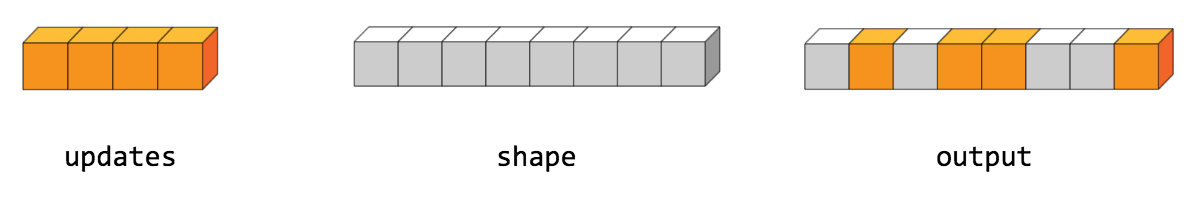
In Scala, this scatter operation would look like this:
val indices = constant(Tensor(Tensor(4), Tensor(3), Tensor(1), Tensor(7)))
val updates = constant(Tensor(9, 10, 11, 12))
val shape = constant(Tensor(8))
scatterND(indices, updates, shape) ==> [0, 11, 0, 10, 9, 0, 0, 12]
We can also, insert entire slices of a higher rank tensor all at once. For example, say we want to insert two
slices in the first dimension of a rank-3 tensor with two matrices of new values.
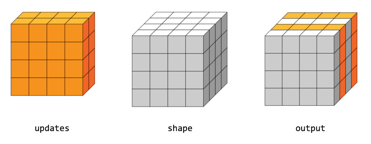
In Scala, this scatter operation would look like this:
val indices = constant(Tensor(Tensor(0), Tensor(2)))
val updates = constant(Tensor(Tensor(Tensor(5, 5, 5, 5), Tensor(6, 6, 6, 6),
                                     Tensor(7, 7, 7, 7), Tensor(8, 8, 8, 8))
                              Tensor(Tensor(5, 5, 5, 5), Tensor(6, 6, 6, 6),
                                     Tensor(7, 7, 7, 7), Tensor(8, 8, 8, 8))))
val shape = constant(Tensor(4, 4, 4))
scatterND(indices, updates, shape) ==>
  [[[5, 5, 5, 5], [6, 6, 6, 6], [7, 7, 7, 7], [8, 8, 8, 8]],
   [[0, 0, 0, 0], [0, 0, 0, 0], [0, 0, 0, 0], [0, 0, 0, 0]],
   [[5, 5, 5, 5], [6, 6, 6, 6], [7, 7, 7, 7], [8, 8, 8, 8]],
   [[0, 0, 0, 0], [0, 0, 0, 0], [0, 0, 0, 0], [0, 0, 0, 0]]]
Indices tensor (must have INT32 or INT64 data type).
Updates to scatter into the output tensor.
One-dimensional INT32 or INT64 tensor specifying the shape of the output tensor.
Name for the created op.
Created op output.
The segmentMax op computes the max along segments of a tensor.
The segmentMax op computes the max along segments of a tensor.
The op computes a tensor such that output(i) = \max_{j...} data(j,...) where the max is over all j
such that segmentIndices(j) == i. Unlike unsortedSegmentMax, segmentIndices need be sorted.
If the max if empty for a given segment index i, output(i) is set to 0.
The result tensor has the same data type as data, but its first dimension size is equal to the number of
distinct segment indices.
Data (must have a numeric data type -- i.e., representing a number).
Segment indices (must have data type of INT32 or INT64). Values should be sorted and can be repeated.
Name for the created op.
Created op output.
The segmentMean op computes the mean along segments of a tensor.
The segmentMean op computes the mean along segments of a tensor.
The op computes a tensor such that output(i) = \frac{sum_{j...} data(j,...)}{N} where the sum is over
all j such that segmentIndices(j) == i and N is the total number of values being summed. Unlike
unsortedSegmentMean, segmentIndices need to be sorted.
If the sum if empty for a given segment index i, output(i) is set to 0.
The result tensor has the same data type as data, but its first dimension size is equal to the number of
distinct segment indices.
Data (must have a numeric data type -- i.e., representing a number).
Segment indices (must have data type of INT32 or INT64). Values should be sorted and can be repeated.
Name for the created op.
Created op output.
The segmentMin op computes the min along segments of a tensor.
The segmentMin op computes the min along segments of a tensor.
The op computes a tensor such that output(i) = \min_{j...} data(j,...) where the min is over all j
such that segmentIndices(j) == i. Unlike unsortedSegmentMin, segmentIndices need be sorted.
If the min if empty for a given segment index i, output(i) is set to 0.
The result tensor has the same data type as data, but its first dimension size is equal to the number of
distinct segment indices.
Data (must have a numeric data type -- i.e., representing a number).
Segment indices (must have data type of INT32 or INT64). Values should be sorted and can be repeated.
Name for the created op.
Created op output.
The segmentProd op computes the product along segments of a tensor.
The segmentProd op computes the product along segments of a tensor.
The op computes a tensor such that output(i) = \prod_{j...} data(j,...) where the product is over all j
such that segmentIndices(j) == i. Unlike unsortedSegmentProd, segmentIndices need be sorted.
If the product if empty for a given segment index i, output(i) is set to 1.
The result tensor has the same data type as data, but its first dimension size is equal to the number of
distinct segment indices.
Data (must have a numeric data type -- i.e., representing a number).
Segment indices (must have data type of INT32 or INT64). Values should be sorted and can be repeated.
Name for the created op.
Created op output.
The segmentSum op computes the sum along segments of a tensor.
The segmentSum op computes the sum along segments of a tensor.
The op computes a tensor such that output(i) = \sum_{j...} data(j,...) where the sum is over all j such
that segmentIndices(j) == i. Unlike unsortedSegmentSum, segmentIndices need be sorted.
If the sum if empty for a given segment index i, output(i) is set to 0.
The result tensor has the same data type as data, but its first dimension size is equal to the number of
distinct segment indices.
Data (must have a numeric data type -- i.e., representing a number).
Segment indices (must have data type of INT32 or INT64). Values should be sorted and can be repeated.
Name for the created op.
Created op output.
The select op selects elements from x or y, depending on condition.
The select op selects elements from x or y, depending on condition.
The x, and y tensors must have the same shape. The output tensor will also have the same shape.
The condition tensor must be a scalar if x and y are scalars. If x and y are vectors or higher rank,
then condition must be either a scalar, or a vector with size matching the first dimension of x, or it must
have the same shape as x.
The condition tensor acts as a mask that chooses, based on the value at each element, whether the
corresponding element / row in the output should be taken from x (if true) or y (if false).
If condition is a vector and x and y are higher rank matrices, then it chooses which row (outer dimension)
to copy from x and y. If condition has the same shape as x and y, then it chooses which element to
copy from x and y.
For example:
// 'condition' tensor is [[true,  false], [false, true]]
// 'x' is [[1, 2], [3, 4]]
// 'y' is [[5, 6], [7, 8]]
select(condition, x, y) ==> [[1, 6], [7, 4]]

// 'condition' tensor is [true, false]
// 'x' is [[1, 2], [3, 4]]
// 'y' is [[5, 6], [7, 8]]
select(condition, x, y) ==> [[1, 2], [7, 8]]
Boolean condition tensor.
Tensor which may have the same shape as condition. If condition has rank 1, then t may
have a higher rank, but its first dimension must match the size of condition.
Tensor with the same data type and shape as t.
Name for the created op.
Created op output.
The selu op computes the scaled exponential linear unit activation function.
The selu op computes the scaled exponential linear unit activation function.
The scaled exponential linear unit activation function is defined as selu(x) = scale * x, if x > 0, and
elu(x) = scale * alpha * (exp(x) - 1), otherwise, where scale = 1.0507 and alpha = 1.7581.
Source: [Self-Normalizing Neural Networks](https://arxiv.org/abs/1706.02515)
Name for the created op.
Created op output.
The sequenceLoss op computes an optionally weighted loss for a sequence of predicted logits.
The sequenceLoss op computes an optionally weighted loss for a sequence of predicted logits.
Depending on the values of averageAcrossTimeSteps and averageAcrossBatch, the returned tensor will have rank
0, 1, or 2 as these arguments reduce the cross-entropy each label, which has shape
[batchSize, sequenceLength], over their respective dimensions. For examplem if averageAcrossTimeSteps is
true and averageAcrossBatch is false, then the returned tensor will have shape [batchSize].
Tensor of shape [batchSize, sequenceLength, numClasses] containing unscaled log
probabilities.
Tensor of shape [batchSize, sequenceLength] containing the true label at each
time step.
Optionally, a tensor of shape [batchSize, sequenceLength] containing weights to
use for each prediction. When using weights as masking, set all valid time steps
to 1 and all padded time steps to 0 (e.g., a mask returned by tf.sequenceMask).
If true, the loss is summed across the sequence dimension and divided by the
total label weight across all time steps.
If true, the loss is summed across the batch dimension and divided by the batch
size.
Loss function to use that takes the predicted logits and the true labels as inputs
and returns the loss value. Defaults to sparseSoftmaxCrossEntropy.
Name prefix to use for the created ops.
Created op output.
InvalidShapeException If any of logits, labels, or weights has invalid shape.
The sequenceMask op returns a mask tensor representing the first N positions of each row of a matrix.
The sequenceMask op returns a mask tensor representing the first N positions of each row of a matrix.
For example:
// 'lengths' = [1, 3, 2]
// 'maxLength' = 5
sequenceMask(lengths, maxLength) ==>
  [[true, false, false, false, false],
   [true,  true,  true, false, false],
   [true,  true, false, false, false]]
One-dimensional integer tensor containing the lengths to keep for each row. If maxLength is
provided, then all values in lengths must be smaller than maxLength.
Scalar integer tensor representing the maximum length of each row. Defaults to the maximum value
in lengths.
Data type for the output tensor.
Name for the created op.
Created op output.
IllegalArgumentException If maxLength is not a scalar.
The setDifference op computes the set difference of elements in the last dimension of a and b.
The setDifference op computes the set difference of elements in the last dimension of a and b.
All but the last dimension of a and b must match.
Note that supported input types are:
(a: SparseOutput, b: SparseOutput)(a: Output, b: SparseOutput)(a: Output, b: Output)For sparse tensors, the indices must be sorted in row-major order.
For example:
val a = SparseOutput(
  indices = Tensor(
    Tensor(0, 0, 0),
    Tensor(0, 0, 1),
    Tensor(0, 1, 0),
    Tensor(1, 0, 0),
    Tensor(1, 1, 0),
    Tensor(1, 1, 1))
  values = Tensor(1, 2, 3, 4, 5, 6),
  denseShape = Shape(2, 2, 2))
val b = SparseOutput(
  indices = Tensor(
    Tensor(0, 0, 0),
    Tensor(0, 0, 1),
    Tensor(0, 1, 0),
    Tensor(1, 0, 0),
    Tensor(1, 0, 1),
    Tensor(1, 1, 0),
    Tensor(1, 1, 1),
    Tensor(1, 1, 2),
    Tensor(1, 1, 3))
  values = Tensor(1, 3, 2, 4, 5, 5, 6, 7, 8),
  denseShape = Shape(2, 2, 4))
tf.setDifference(a, b) ==>
  SparseTensor(
    indices = Tensor(
      Tensor(0, 0, 0),
      Tensor(0, 0, 1)),
    values = Tensor(2, 3))
First input tensor.
Second input tensor.
Boolean value specifying whether to subtract b from a, or vice-versa.
Boolean indicator specifying whether to validate the order and range of the indices of
input.
Name for the created op.
Sparse tensor containing the result of the operation.
InvalidDataTypeException If any of the input tensors has an unsupported data type.
The setIntersection op computes the set intersection of elements in the last dimension of a and b.
The setIntersection op computes the set intersection of elements in the last dimension of a and b.
All but the last dimension of a and b must match.
Note that supported input types are:
(a: SparseOutput, b: SparseOutput)(a: Output, b: SparseOutput)(a: Output, b: Output)For sparse tensors, the indices must be sorted in row-major order.
For example:
val a = SparseOutput(
  indices = Tensor(
    Tensor(0, 0, 0),
    Tensor(0, 0, 1),
    Tensor(0, 1, 0),
    Tensor(1, 0, 0),
    Tensor(1, 1, 0),
    Tensor(1, 1, 1))
  values = Tensor(1, 2, 3, 4, 5, 6),
  denseShape = Shape(2, 2, 2))
val b = SparseOutput(
  indices = Tensor(
    Tensor(0, 0, 0),
    Tensor(1, 0, 0),
    Tensor(1, 1, 0),
    Tensor(1, 1, 1),
    Tensor(1, 1, 2),
    Tensor(1, 1, 3))
  values = Tensor(1, 4, 5, 6, 7, 8),
  denseShape = Shape(2, 2, 4))
tf.setIntersection(a, b) ==>
  SparseTensor(
    indices = Tensor(
      Tensor(0, 0, 0),
      Tensor(1, 0, 0),
      Tensor(1, 1, 0),
      Tensor(1, 1, 1)),
    values = Tensor(1, 4, 5, 6))
First input tensor.
Second input tensor.
Boolean indicator specifying whether to validate the order and range of the indices of
input.
Name for the created op.
Sparse tensor containing the result of the operation.
InvalidDataTypeException If any of the input tensors has an unsupported data type.
The setSize op computes the number of unique elements along the last dimension of input.
The setSize op computes the number of unique elements along the last dimension of input.
For input with rank n, the op outputs a tensor with rank n-1, and the same 1st n-1 dimensions as
input. Each value is the number of unique elements in the corresponding [0, ..., n-1] dimension of input.
Input tensor with indices sorted in row-major order.
Boolean indicator specifying whether to validate the order and range of the indices of
input.
Name for the created op.
INT32 tensor containing the set sizes.
InvalidDataTypeException If input has an unsupported data type.
The setUnion op computes the set union of elements in the last dimension of a and b.
The setUnion op computes the set union of elements in the last dimension of a and b.
All but the last dimension of a and b must match.
Note that supported input types are:
(a: SparseOutput, b: SparseOutput)(a: Output, b: SparseOutput)(a: Output, b: Output)For sparse tensors, the indices must be sorted in row-major order.
For example:
val a = SparseOutput(
  indices = Tensor(
    Tensor(0, 0, 0),
    Tensor(0, 0, 1),
    Tensor(0, 1, 0),
    Tensor(1, 0, 0),
    Tensor(1, 1, 0),
    Tensor(1, 1, 1))
  values = Tensor(1, 2, 3, 4, 5, 6),
  denseShape = Shape(2, 2, 2))
val b = SparseOutput(
  indices = Tensor(
    Tensor(0, 0, 0),
    Tensor(0, 0, 1),
    Tensor(0, 1, 0),
    Tensor(1, 0, 0),
    Tensor(1, 0, 1),
    Tensor(1, 1, 0),
    Tensor(1, 1, 1),
    Tensor(1, 1, 2),
    Tensor(1, 1, 3))
  values = Tensor(1, 3, 2, 4, 5, 5, 6, 7, 8),
  denseShape = Shape(2, 2, 4))
tf.setDifference(a, b) ==>
  SparseTensor(
    indices = Tensor(
    Tensor(0, 0, 0),
    Tensor(0, 0, 1),
    Tensor(0, 0, 2),
    Tensor(0, 1, 0),
    Tensor(1, 0, 0),
    Tensor(1, 0, 1),
    Tensor(1, 1, 0),
    Tensor(1, 1, 1),
    Tensor(1, 1, 2),
    Tensor(1, 1, 3))
  values = Tensor(1, 2, 3, 2, 3, 4, 5, 5, 6, 7, 8))
First input tensor.
Second input tensor.
Boolean indicator specifying whether to validate the order and range of the indices of
input.
Name for the created op.
Sparse tensor containing the result of the operation.
InvalidDataTypeException If any of the input tensors has an unsupported data type.
The shape op returns the shape of a tensor.
The shape op returns the shape of a tensor.
The op returns a one-dimensional tensor representing the shape of input.
For example:
// 't' is [[[1, 1, 1], [2, 2, 2]], [[3, 3, 3], [4, 4, 4]]]
shape(t) ==> [2, 2, 3]
Tensor whose shape to return.
Optional data type to use for the output of this op.
Boolean flag indicating whether to optimize this op creation by using a constant op with the
shape of that input at graph creation time (instead of execution time), if known.
Name for the created op.
Created op output, which is one-dimensional.
The shapeN op returns the shape of an array of tensors.
The shapeN op returns the shape of an array of tensors.
The op returns an array of one-dimensional tensors, each one representing the shape of the corresponding tensor
in inputs.
Tensors whose shapes to return.
Optional data type to use for the outputs of this op.
Name for the created op.
Created op outputs, all of which are one-dimensional.
Returns the set of all shared resources used by the current graph which need to be initialized once per cluster.
Returns the set of all shared resources used by the current graph which need to be initialized once per cluster.
Returns an initializer op for all shared resources that have been created in the current graph.
Returns an initializer op for all shared resources that have been created in the current graph.
The sigmoid op computes the sigmoid function element-wise on a tensor.
The sigmoid op computes the sigmoid function element-wise on a tensor.
Specifically, y = 1 / (1 + exp(-x)).
Input tensor that must be one of the following types: HALF, FLOAT32, FLOAT64, INT32, INT64,
COMPLEX64, or COMPLEX128.
Name for the created op.
Created op output.
The sigmoidCrossEntropy op computes the sigmoid cross entropy between logits and labels.
The sigmoidCrossEntropy op computes the sigmoid cross entropy between logits and labels.
The op measures the probability error in discrete classification tasks in which each class is independent and not mutually exclusive. For instance, one could perform multi-label classification where a picture can contain both an elephant and a dog at the same time.
For brevity, let x = logits and z = labels. The sigmoid cross entropy (also known as logistic loss) is
defined as:
z * -log(sigmoid(x)) + (1 - z) * -log(1 - sigmoid(x))
= z * -log(1 / (1 + exp(-x))) + (1 - z) * -log(exp(-x) / (1 + exp(-x)))
= z * log(1 + exp(-x)) + (1 - z) * (-log(exp(-x)) + log(1 + exp(-x)))
= z * log(1 + exp(-x)) + (1 - z) * (x + log(1 + exp(-x))
= (1 - z) * x + log(1 + exp(-x))
= x - x * z + log(1 + exp(-x))
For x < 0, to avoid numerical overflow in exp(-x), we reformulate the above to:
x - x * z + log(1 + exp(-x))
= log(exp(x)) - x * z + log(1 + exp(-x))
= - x * z + log(1 + exp(x))
Hence, to ensure stability and avoid numerical overflow, the implementation uses this equivalent formulation:
max(x, 0) - x * z + log(1 + exp(-abs(x)))
If weights is not null, then the positive examples are weighted. A value weights > 1 decreases the false
negative count, hence increasing recall. Conversely setting weights < 1 decreases the false positive count and
increases precision. This can be seen from the fact that weight is introduced as a multiplicative coefficient
for the positive targets term in the loss expression (where q = weights, for brevity):
qz * -log(sigmoid(x)) + (1 - z) * -log(1 - sigmoid(x))
= qz * -log(1 / (1 + exp(-x))) + (1 - z) * -log(exp(-x) / (1 + exp(-x)))
= qz * log(1 + exp(-x)) + (1 - z) * (-log(exp(-x)) + log(1 + exp(-x)))
= qz * log(1 + exp(-x)) + (1 - z) * (x + log(1 + exp(-x))
= (1 - z) * x + (qz + 1 - z) * log(1 + exp(-x))
= (1 - z) * x + (1 + (q - 1) * z) * log(1 + exp(-x))
Setting l = 1 + (q - 1) * z, to ensure stability and avoid numerical overflow, the implementation uses this
equivalent formulation:
(1 - z) * x + l * (max(-x, 0) + log(1 + exp(-abs(x))))
logits and labels must have the same shape.
Tensor of shape [D0, D1, ..., Dr-1, numClasses] and data type FLOAT16, FLOAT32, or
FLOAT64, containing unscaled log probabilities.
Tensor of shape [D0, D1, ..., Dr-1, numClasses] and data type FLOAT16, FLOAT32, or
FLOAT64, where each row must be a valid probability distribution.
Optionally, a coefficient to use for the positive examples.
Name for the created op.
Created op output, with rank one less than that of logits and the same data type as logits, containing
the sigmoid cross entropy loss.
The sign op computes an element-wise indication of the sign of a tensor.
The sign op computes an element-wise indication of the sign of a tensor.
I.e., y = sign(x) = -1 if x < 0; 0 if x == 0; 1 if x > 0.
Zero is returned for NaN inputs.
For complex numbers, y = sign(x) = x / |x| if x != 0, otherwise y = 0.
Input tensor that must be one of the following types: HALF, FLOAT32, FLOAT64, INT32, INT64,
COMPLEX64, or COMPLEX128.
Name for the created op.
Created op output.
The sin op computes the sine of a tensor element-wise.
The sin op computes the sine of a tensor element-wise. I.e., y = \sin{x}.
Input tensor that must be one of the following types: HALF, FLOAT32, FLOAT64, INT32, INT64,
COMPLEX64, or COMPLEX128.
Name for the created op.
Created op output.
The sinh op computes the hyperbolic sine of a tensor element-wise.
The sinh op computes the hyperbolic sine of a tensor element-wise. I.e., y = \sinh{x}.
Input tensor that must be one of the following types: HALF, FLOAT32, FLOAT64, INT32, INT64,
COMPLEX64, or COMPLEX128.
Name for the created op.
Created op output.
The size op returns the size of a tensor.
The size op returns the size of a tensor.
The op returns a number representing the number of elements in input.
For example:
// 't' is [[[1, 1, 1], [2, 2, 2]], [[3, 3, 3], [4, 4, 4]]]]
size(t) ==> 12
Tensor whose size to return.
Optional data type to use for the output of this op.
Boolean flag indicating whether to optimize this op creation by using a constant op with the
number of elements provided by the shape of that input at graph creation time (instead of
execution time), if known.
Name for the created op.
Created op output.
The slice op returns a slice from input.
The slice op returns a slice from input.
The op output is a tensor with dimensions described by size, whose values are extracted from input, starting
at the offsets in begin.
Requirements:
0 <= begin(i) <= begin(i) + size(i) <= Di, for i in [0, n), where Di corresponds to the size of
the ith dimension of input and n corresponds to the rank of input.Tensor to slice.
Begin index tensor (must have data type of INT32 or INT64). begin(i) specifies the offset into
the ith dimension of input to slice from.
Slice size tensor (must have data type of INT32 or INT64). size(i) specifies the number of
elements of the ith dimension of input to slice. If size(i) == -1, then all the remaining
elements in dimension i are included in the slice (i.e., this is equivalent to setting
size(i) = input.shape(i) - begin(i)).
Name for the created op.
Created op output.
The softmax op computes softmax activations.
The softmax op computes softmax activations.
For each batch i and class j we have softmax = exp(logits) / sum(exp(logits), axis), where axis
indicates the axis the softmax should be performed on.
Tensor containing the logits with data type FLOAT16, FLOAT32, or FLOAT64.
Axis along which to perform the softmax. Defaults to -1 denoting the last axis.
Name for the created op.
Created op output.
The softmaxCrossEntropy op computes the softmax cross entropy between logits and labels.
The softmaxCrossEntropy op computes the softmax cross entropy between logits and labels.
The op measures the probabilistic error in discrete classification tasks in which the classes are mutually exclusive (each entry belongs to exactly one class). For example, each CIFAR-10 image is labeled with one and only one label: an image can be a dog or a truck, but not both.
Back-propagation will happen into both logits and labels. To disallow back-propagation into labels, pass
the label tensors through a stopGradients op before feeding it to this function.
NOTE: While the classes are mutually exclusive, their probabilities need not be. All that is required is
that each row of labels is a valid probability distribution. If they are not, the computation of the gradient
will be incorrect. If using exclusive labels (wherein one and only one class is true at a time), see
sparseSoftmaxCrossEntropy.
WARNING: The op expects unscaled logits, since it performs a softmax on logits internally for
efficiency. Do not call this op with the output of softmax, as it will produce incorrect results.
logits and labels must have the same shape. A common use case if to have logits and labels of shape
[batchSize, numClasses], but higher dimensions are also supported.
logits and labels must have data type FLOAT16, FLOAT32, or FLOAT64.
Tensor of shape [D0, D1, ..., Dr-1, numClasses] and data type FLOAT16, FLOAT32, or
FLOAT64, containing unscaled log probabilities.
Tensor of shape [D0, D1, ..., Dr-1, numClasses] and data type FLOAT16, FLOAT32, or
FLOAT64, where each row must be a valid probability distribution.
The class axis, along which the softmax is computed. Defaults to -1, which is the last axis.
Name for the created op.
Created op output, with rank one less than that of logits and the same data type as logits, containing
the softmax cross entropy loss.
The softplus op computes the softplus activation function.
The softplus op computes the softplus activation function.
The softplus activation function is defined as softplus(x) = log(exp(x) + 1).
Name for the created op.
Created op output.
The softsign op computes the softsign activation function.
The softsign op computes the softsign activation function.
The softsign activation function is defined as softsign(x) = x / (abs(x) + 1).
Name for the created op.
Created op output.
The spaceToBatch op zero-pads and then rearranges (permutes) blocks of spatial data into batches.
The spaceToBatch op zero-pads and then rearranges (permutes) blocks of spatial data into batches.
More specifically, the op outputs a copy of the input tensor where values from the height and width
dimensions are moved to the batch dimension. After the zero-padding, both height and width of the input
must be divisible by blockSize (which must be greater than 1). This is the reverse functionality to that of
batchToSpace.
input is a 4-dimensional input tensor with shape [batch, height, width, depth].
paddings has shape [2, 2]. It specifies the padding of the input with zeros across the spatial dimensions as
follows: paddings = padBottom], [padLeft, padRight. The effective spatial dimensions of the
zero-padded input tensor will be:
heightPad = padTop + height + padBottomwidthPad = padLeft + width + padRight blockSize indicates the block size:
blockSize x blockSize in the height and width dimensions are rearranged
into the batch dimension at each location.batch * blockSize * blockSize.heightPad and widthPad must be divisible by blockSize. The shape of the output will be:
[batch * blockSize * blockSize, heightPad / blockSize, widthPad / blockSize, depth]
Some examples:
// === Example #1 ===
// input = [[[[1], [2]], [[3], [4]]]]  (shape = [1, 2, 2, 1])
// blockSize = 2
// paddings = [[0, 0], [0, 0]]
spaceToBatch(input, blockSize, paddings) ==> [[[[1]]], [[[2]]], [[[3]]], [[[4]]]]  (shape = [4, 1, 1, 1])

// === Example #2 ===
// input = [[[[1, 2, 3], [4,   5,  6]],
//           [[7, 8, 9], [10, 11, 12]]]]  (shape = [1, 2, 2, 3])
// blockSize = 2
// paddings = [[0, 0], [0, 0]]
spaceToBatch(input, blockSize, paddings) ==>
  [[[1, 2, 3]], [[4, 5, 6]], [[7, 8, 9]], [[10, 11, 12]]]  (shape = [4, 1, 1, 3])

// === Example #3 ===
// input = [[[[ 1],  [2],  [3],  [ 4]],
//           [[ 5],  [6],  [7],  [ 8]],
//           [[ 9], [10], [11],  [12]],
//           [[13], [14], [15],  [16]]]]  (shape = [1, 4, 4, 1])
// blockSize = 2
// paddings = [[0, 0], [0, 0]]
spaceToBatch(input, blockSize, paddings) ==>
  [[[[1], [3]], [[ 9], [11]]],
   [[[2], [4]], [[10], [12]]],
   [[[5], [7]], [[13], [15]]],
   [[[6], [8]], [[14], [16]]]]  (shape = [4, 2, 2, 1])

// === Example #4 ===
// input = [[[[ 1],  [2],  [3],  [ 4]],
//           [[ 5],  [6],  [7],  [ 8]]],
//          [[[ 9], [10], [11],  [12]],
//           [[13], [14], [15],  [16]]]]  (shape = [2, 2, 4, 1])
// blockSize = 2
// paddings = [[0, 0], [2, 0]]
spaceToBatch(input, blockSize, paddings) ==>
  [[[[0], [1], [3]]], [[[0], [ 9], [11]]],
   [[[0], [2], [4]]], [[[0], [10], [12]]],
   [[[0], [5], [7]]], [[[0], [13], [15]]],
   [[[0], [6], [8]]], [[[0], [14], [16]]]]  (shape = [8, 1, 3, 1])
4-dimensional input tensor with shape [batch, height, width, depth].
Block size which must be greater than 1.
2-dimensional INT32 or INT64 tensor containing non-negative integers with shape
[2, 2].
Name for the created op.
Created op output.
The spaceToBatchND op divides "spatial" dimensions [1, ..., M] of input into a grid of blocks with shape
blockShape, and interleaves these blocks with the "batch" dimension (0) such that, in the output, the
spatial dimensions [1, ..., M] correspond to the position within the grid, and the batch dimension combines
both the position within a spatial block and the original batch position.
The spaceToBatchND op divides "spatial" dimensions [1, ..., M] of input into a grid of blocks with shape
blockShape, and interleaves these blocks with the "batch" dimension (0) such that, in the output, the
spatial dimensions [1, ..., M] correspond to the position within the grid, and the batch dimension combines
both the position within a spatial block and the original batch position. Prior to division into blocks, the
spatial dimensions of the input are optionally zero padded according to paddings. This is the reverse
functionality to that of batchToSpaceND.
input is an N-dimensional tensor with shape inputShape = [batch] + spatialShape + remainingShape, where
spatialShape has M dimensions.
The op is equivalent to the following steps:
paddedShape.
2. Reshape padded to reshapedPadded of shape:[batch] + [[paddedShape(1) / blockShape(0), blockShape(0), ..., paddedShape(M) / blockShape(M-1), blockShape(M-1)]` + remainingShape
3. Permute the dimensions of reshapedPadded to produce permutedReshapedPadded of shape:
blockShape +
[batch] +
[paddedShape(1) / blockShape(0), ..., paddedShape(M) / blockShape(M-1)] +
remainingShape
4. Reshape permutedReshapedPadded to flatten blockShape into the batch dimension, producing an output
tensor of shape:
[batch *   product(blockShape)] +
[paddedShape(1) / blockShape(0), ..., paddedShape(M) / blockShape(M-1)] +
remainingShape
Among others, this op is useful for reducing atrous convolution to regular convolution.
Some examples:
// === Example #1 ===
// input = [[[[1], [2]], [[3], [4]]]]  (shape = [1, 2, 2, 1])
// blockShape = [2, 2]
// paddings = [[0, 0], [0, 0]]
spaceToBatchND(input, blockShape, paddings) ==>
  [[[[1]]], [[[2]]], [[[3]]], [[[4]]]]  (shape = [4, 1, 1, 1])

// === Example #2 ===
// input = [[[[1, 2, 3], [4, 5, 6]],
//           [[7, 8, 9], [10, 11, 12]]]]  (shape = [1, 2, 2, 3])
// blockShape = [2, 2]
// paddings = [[0, 0], [0, 0]]
spaceToBatchND(input, blockShape, paddings) ==>
  [[[1, 2, 3]], [[4, 5, 6]], [[7, 8, 9]], [[10, 11, 12]]]  (shape = [4, 1, 1, 3])

// === Example #3 ===
// input = [[[[ 1],  [2],  [3],  [ 4]],
//           [[ 5],  [6],  [7],  [ 8]],
//           [[ 9], [10], [11],  [12]],
//           [[13], [14], [15],  [16]]]]  (shape = [1, 4, 4, 1])
// blockShape = [2, 2]
// paddings = [[0, 0], [0, 0]]
spaceToBatchND(input, blockShape, paddings) ==>
  [[[[1], [3]], [[ 9], [11]]],
   [[[2], [4]], [[10], [12]]],
   [[[5], [7]], [[13], [15]]],
   [[[6], [8]], [[14], [16]]]]  (shape = [4, 2, 2, 1])

// === Example #4 ===
// input = [[[[ 1],  [2],  [3],  [ 4]],
//           [[ 5],  [6],  [7],  [ 8]]],
//          [[[ 9], [10], [11],  [12]],
//           [[13], [14], [15],  [16]]]]  (shape = [2, 2, 4, 1])
// blockShape = [2, 2]
// paddings = [[0, 0], [2, 0]]
spaceToBatchND(input, blockShape, paddings) ==>
  [[[[0], [1], [3]]], [[[0], [ 9], [11]]],
   [[[0], [2], [4]]], [[[0], [10], [12]]],
   [[[0], [5], [7]]], [[[0], [13], [15]]],
   [[[0], [6], [8]]], [[[0], [14], [16]]]]  (shape = [8, 1, 3, 1])
N-dimensional tensor with shape inputShape = [batch] + spatialShape + remainingShape, where
spatialShape has M dimensions.
One-dimensional INT32 or INT64 tensor with shape [M] whose elements must all be
>= 1.
Two-dimensional INT32 or INT64 tensor with shape [M, 2] whose elements must all be
non-negative. paddings(i) = [padStart, padEnd] specifies the padding for input dimension
i + 1, which corresponds to spatial dimension i. It is required that blockShape(i)
divides inputShape(i + 1) + padStart + padEnd.
Name for the created op.
Created op output.
The spaceToDepth op that rearranges blocks of spatial data, into depth.
The spaceToDepth op that rearranges blocks of spatial data, into depth.
More specifically, the op outputs a copy of the input tensor where values from the height and width
dimensions are moved to the depth dimension. blockSize indicates the input block size and how the data is
moved:
blockSize x blockSize in the height and width dimensions are rearranged
into the depth dimension at each location.inputDepth * blockSize * blockSize.height and width must be divisible by blockSize. That is, assuming that input is in the shape [batch, height, width, depth], the shape of the output will be:
[batch, height / blockSize, width / blockSize, depth * block_size * block_size].
This op is useful for resizing the activations between convolutions (but keeping all data), e.g., instead of pooling. It is also useful for training purely convolutional models.
Some examples:
// === Example #1 ===
// input = [[[[1], [2]], [[3], [4]]]]  (shape = [1, 2, 2, 1])
// blockSize = 2
spaceToDepth(input, blockSize) ==> [[[[1, 2, 3, 4]]]]  (shape = [1, 1, 1, 4])

// === Example #2 ===
// input =  [[[[1, 2, 3], [4, 5, 6]], [[7, 8, 9]], [[10, 11, 12]]]  (shape = [1, 2, 2, 3])
// blockSize = 2
spaceToDepth(input, blockSize) ==>
  [[[[1, 2, 3, 4, 5, 6, 7, 8, 9, 10, 11, 12]]]]  (shape = [1, 1, 1, 12])

// === Example #3 ===
// input = [[[[ 1], [ 2], [ 5], [ 6]],
//           [[ 3], [ 4], [ 7], [ 8]],
//           [[ 9], [10], [13], [14]],
//           [[11], [12], [15], [16]]]]  (shape = [1, 4, 4, 1])
// blockSize = 2
spaceToDepth(input, blockSize) ==>
  [[[[ 1,  2,  3,  4],
     [ 5,  6,  7,  8]],
    [[ 9, 10, 11, 12],
     [13, 14, 15, 16]]]]  (shape = [1, 2, 2, 4])
4-dimensional input tensor with shape [batch, height, width, depth].
Block size which must be greater than 1.
Format of the input and output data.
Name for the created op.
Created op output.
The sparseEmbeddingLookup op looks up and computes embeddings for the given sparse ids and weights.
The sparseEmbeddingLookup op looks up and computes embeddings for the given sparse ids and weights.
The op assumes that there is at least one id for each row in the dense tensor represented by sparseIds (i.e.,
there are no rows with empty features), and that all the indices of sparseIds are in canonical row-major
order. It also assumes that all id values lie in the range [0, p0), where p0 is the sum of the size of
parameters along dimension 0.
The op returns a dense tensor representing the combined embeddings for the provided sparse ids. For each row in
the dense tensor represented by sparseIds, the op looks up the embeddings for all ids in that row, multiplies
them by the corresponding weight, and combines them using the provided combiner.
In other words, if shape(combinedParameters) = [p0, p1, ..., pm] and
shape(sparseIds) = shape(sparseWeights) = [d0, d1, ..., dn], then
shape(output) = [d0, d1, ..., dn-1, p1, ..., pm].
For instance, if parameters is a 10x20 matrix, and sparseIds and sparseWeights are as follows:
and we are using the MeanCombiner, then the output will be a 3x20 matrix, where:
Embedding map, which is either a single tensor, a list of P tensors with the same
shape, except for their first dimension, representing sharded embedding tensors, or a
PartitionedVariable, created by partitioning along the first dimension.
NxM sparse tensor containing INT64 ids, where N typically corresponds to the batch
size and M is arbitrary.
Either a sparse tensor containing FLOAT32 or FLOAT64 weight values, or None null
to indicate all weights should be taken to be equal to 1. If specified, sparseWeights
must have exactly the same shape and indices as sparseIds.
Partitioning strategy to use if parameters.numPartitions > 1.
Combination/reduction strategy to use for the obtained embeddings.
If provided, embedding values are l2-normalized to this value.
Name prefix used for the created op.
Obtained embeddings for the provided ids.
The sparsePlaceholder op returns a placeholder for a sparse tensor that will always be fed.
The sparsePlaceholder op returns a placeholder for a sparse tensor that will always be fed.
IMPORTANT NOTE: This op will produce an error if evaluated. Its value must be fed when using
Session.run. It is intended as a way to represent a value that will always be fed, and to provide attributes
that enable the fed value to be checked at runtime.
Data type of the elements in the tensor that will be fed.
Shape of the tensor that will be fed. The shape can be any partially-specified, or even completely unknown. This represents the shape of the dense tensor that corresponds to the sparse tensor that this placeholder refers to.
Name for the created op.
Created op output.
The sparseSegmentMean op computes the mean along sparse segments of a tensor.
The sparseSegmentMean op computes the mean along sparse segments of a tensor.
The op is similar to that of segmentMean, with the difference that segmentIndices can have rank less
than data's first dimension, selecting a subset of dimension 0, specified by indices. segmentIndices is
allowed to have missing indices, in which case the output will be zeros at those indices. In those cases,
numSegments is used to determine the size of the output.
For example:
// 'c' is [[1, 2, 3, 4], [-1, -2, -3, -4], [5, 6, 7, 8]]

// Select two rows, one segment.
sparseSegmentMean(c, Tensor(0, 1), Tensor(0, 0)) ==> [[0, 0, 0, 0]]

// Select two rows, two segments.
sparseSegmentMean(c, Tensor(0, 1), Tensor(0, 1)) ==> [[1, 2, 3, 4], [-1, -2, -3, -4]]

// Select all rows, two segments.
sparseSegmentMean(c, Tensor(0, 1, 2), Tensor(0, 0, 1)) ==> [[0, 0, 0, 0], [5, 6, 7, 8]]
// which is equivalent to:
segmentMean(c, Tensor(0, 0, 1))
The result tensor has the same data type as data, but its first dimension size is equal to the number of
distinct segment indices.
Data (must have a numeric data type -- i.e., representing a number).
One-dimensional tensor with rank equal to that of segmentIndices.
Segment indices (must have data type of INT32 or INT64). Values should be sorted and can be repeated.
Optional INT32 scalar indicating the size of the output tensor.
Name for the created op.
Created op output.
The sparseSegmentSum op computes the sum along sparse segments of a tensor.
The sparseSegmentSum op computes the sum along sparse segments of a tensor.
The op is similar to that of segmentSum, with the difference that segmentIndices can have rank less
than data's first dimension, selecting a subset of dimension 0, specified by indices. segmentIndices is
allowed to have missing indices, in which case the output will be zeros at those indices. In those cases,
numSegments is used to determine the size of the output.
For example:
// 'c' is [[1, 2, 3, 4], [-1, -2, -3, -4], [5, 6, 7, 8]]

// Select two rows, one segment.
sparseSegmentSum(c, Tensor(0, 1), Tensor(0, 0)) ==> [[0, 0, 0, 0]]

// Select two rows, two segments.
sparseSegmentSum(c, Tensor(0, 1), Tensor(0, 1)) ==> [[1, 2, 3, 4], [-1, -2, -3, -4]]

// Select all rows, two segments.
sparseSegmentSum(c, Tensor(0, 1, 2), Tensor(0, 0, 1)) ==> [[0, 0, 0, 0], [5, 6, 7, 8]]
// which is equivalent to:
segmentSum(c, Tensor(0, 0, 1))
The result tensor has the same data type as data, but its first dimension size is equal to the number of
distinct segment indices.
Data (must have a numeric data type -- i.e., representing a number).
One-dimensional tensor with rank equal to that of segmentIndices.
Segment indices (must have data type of INT32 or INT64). Values should be sorted and can be repeated.
Optional INT32 scalar indicating the size of the output tensor.
Name for the created op.
Created op output.
The sparseSegmentSumSqrtN op computes the sum along sparse segments of a tensor, divided by the square
root of the number of elements being summed.
The sparseSegmentSumSqrtN op computes the sum along sparse segments of a tensor, divided by the square
root of the number of elements being summed. segmentIndices is allowed to have missing indices, in which case
the output will be zeros at those indices. In those cases, numSegments is used to determine the size of the
output.
Similar to sparseSegmentSum.
The result tensor has the same data type as data, but its first dimension size is equal to the number of
distinct segment indices.
Data (must have a numeric data type -- i.e., representing a number).
One-dimensional tensor with rank equal to that of segmentIndices.
Segment indices (must have data type of INT32 or INT64). Values should be sorted and can be repeated.
Optional INT32 scalar indicating the size of the output tensor.
Name for the created op.
Created op output.
The sparseSoftmaxCrossEntropy op computes the sparse softmax cross entropy between logits and labels.
The sparseSoftmaxCrossEntropy op computes the sparse softmax cross entropy between logits and labels.
The op measures the probabilistic error in discrete classification tasks in which the classes are mutually exclusive (each entry belongs to exactly one class). For example, each CIFAR-10 image is labeled with one and only one label: an image can be a dog or a truck, but not both.
NOTE: For the op, the probability of a given label is considered exclusive. That is, soft classes are not
allowed, and the labels vector must provide a single specific index for the true class for each row of
logits (i.e., each batch instance). For soft softmax classification with a probability distribution for each
entry, see softmaxCrossEntropy.
WARNING: The op expects unscaled logits, since it performs a softmax on logits internally for
efficiency. Do not call this op with the output of softmax, as it will produce incorrect results.
A common use case if to have logits of shape [batchSize, numClasses] and labels of shape [batchSize],
but higher dimensions are also supported.
logits must have data type FLOAT16, FLOAT32, or FLOAT64, and labels must have data type
INT32 or INT64.
Tensor of shape [D0, D1, ..., Dr-1, numClasses] (where r is the rank of labels and of the
result) and data type FLOAT16, FLOAT32, or FLOAT64, containing unscaled log
probabilities.
Tensor of shape [D0, D1, ..., Dr-1] (where r is the rank of labels and of the result) and
data type INT32 or INT64. Each entry in labels must be an index in [0, numClasses).
Other values will raise an exception when this op is run on a CPU, and return NaN values for the
corresponding loss and gradient rows when this op is run on a GPU.
The class axis, along which the softmax is computed. Defaults to -1, which is the last axis.
Name for the created op.
Created op output, with the same shape as labels and the same data type as logits, containing the
softmax cross entropy loss.
The split op splits a tensor into sub-tensors.
The split op splits a tensor into sub-tensors.
The op splits input along dimension axis into splitSizes.length smaller tensors. The shape of the i-th
smaller tensor has the same size as the input except along dimension axis where the size is equal to
splitSizes(i).
For example:
// 't' is a tensor with shape [5, 30]
// Split 't' into 3 tensors with sizes [4, 5, 11] along dimension 1:
val splits = split(t, splitSizes = [4, 15, 11], axis = 1)
splits(0).shape ==> [5, 4]
splits(1).shape ==> [5, 15]
splits(2).shape ==> [5, 11]
Input tensor to split.
Sizes for the splits to obtain.
Dimension along which to split the input tensor.
Name for the created op.
Created op outputs.
The splitEvenly op splits a tensor into sub-tensors.
The splitEvenly op splits a tensor into sub-tensors.
The op splits input along dimension axis into numSplits smaller tensors. It requires that numSplits
evenly splits input.shape(axis).
For example:
// 't' is a tensor with shape [5, 30]
// Split 't' into 3 tensors along dimension 1:
val splits = split(t, numSplits = 3, axis = 1)
splits(0).shape ==> [5, 10]
splits(1).shape ==> [5, 10]
splits(2).shape ==> [5, 10]
Input tensor to split.
Number of splits to obtain along the axis dimension.
Dimension along which to split the input tensor.
Name for the created op.
Created op outputs.
The sqrt op computes the square root of a tensor element-wise.
The sqrt op computes the square root of a tensor element-wise. I.e., y = \sqrt{x} = x^{1/2}.
Input tensor that must be one of the following types: HALF, FLOAT32, FLOAT64, INT32, INT64,
COMPLEX64, or COMPLEX128.
Name for the created op.
Created op output.
The square op computes the square of a tensor element-wise.
The square op computes the square of a tensor element-wise. I.e., y = x * x = x^2.
Input tensor that must be one of the following types: HALF, FLOAT32, FLOAT64, INT32, INT64,
COMPLEX64, or COMPLEX128.
Name for the created op.
Created op output.
The squaredDifference op computes the squared difference between two tensors element-wise.
The squaredDifference op computes the squared difference between two tensors element-wise.
I.e., z = (x - y) * (x - y).
NOTE: This op supports broadcasting. More information about broadcasting can be found [here](http://docs.scipy.org/doc/numpy/user/basics.broadcasting.html).
First input tensor that must be one of the following types: HALF, FLOAT32, FLOAT64, INT32,
INT64, COMPLEX64, or COMPLEX128.
Second input tensor that must be one of the following types: HALF, FLOAT32, FLOAT64, INT32,
INT64, COMPLEX64, or COMPLEX128.
Name for the created op.
Created op output.
The squeeze op removes dimensions of size 1 from the shape of a tensor and returns the result as a new tensor.
The squeeze op removes dimensions of size 1 from the shape of a tensor and returns the result as a new tensor.
Given a tensor input, the op returns a tensor of the same data type, with all dimensions of size 1 removed.
If axes is specified, then only the dimensions specified by that array will be removed. In that case, all
these dimensions need to have size 1.
For example:
// 't' is a tensor of shape [1, 2, 1, 3, 1, 1]
t.squeeze().shape == Shape(2, 3)
t.squeeze(Array(2, 4)).shape == Shape(1, 2, 3, 1)
Input tensor.
Dimensions of size 1 to squeeze. If this argument is not provided, then all dimensions of size 1 will be squeezed.
Name for the created op.
Created op output.
The stack op stacks a list of rank-R tensors into one rank-(R+1) tensor.
The stack op stacks a list of rank-R tensors into one rank-(R+1) tensor.
The op packs the list of tensors in inputs into a tensor with rank one higher than each tensor in inputs, by
packing them along the axis dimension. Given a list of N tensors of shape [A, B, C]:
axis == 0, then the output tensor will have shape [N, A, B, C].axis == 1, then the output tensor will have shape [A, N, B, C].axis == -1, then the output tensor will have shape [A, B, C, N].For example:
// 'x' is [1, 4]
// 'y' is [2, 5]
// 'z' is [3, 6]
stack(Array(x, y, z)) ==> [[1, 4], [2, 5], [3, 6]]          // Packed along the first dimension.
stack(Array(x, y, z), axis = 1) ==> [[1, 2, 3], [4, 5, 6]]  // Packed along the second dimension.
This op is the opposite of unstack.
Input tensors to be stacked.
Dimension along which to stack the input tensors.
Name for the created op.
Created op output.
Creates an op that deletes a stack from its resource container.
Creates an op that deletes a stack from its resource container.
Handle to a stack resource.
Name for the created op.
Created op.
Creates an op that pops an element from a stack and then returns it.
Creates an op that pops an element from a stack and then returns it.
Handle to a stack resource.
Data type of the elements in the stack.
Name for the created op.
Created op output.
Creates an op that pushes an element into a stack and then returns that same element.
Creates an op that pushes an element into a stack and then returns that same element.
Handle to a stack resource.
Element to push into the stack.
Boolean value indicating whether to swap the element memory to the CPU.
Name for the created op.
Created op output, which has the same value as element.
The stopGradient op stops gradient execution, but otherwise acts as an identity op.
The stopGradient op stops gradient execution, but otherwise acts as an identity op.
When executed in a graph, this op outputs its input tensor as-is.
When building ops to compute gradients, this op prevents the contribution of its inputs to be taken into account. Normally, the gradient generator adds ops to a graph to compute the derivatives of a specified 'loss' by recursively finding out inputs that contributed to its computation. If you insert this op in the graph its inputs are masked from the gradient generator. They are not taken into account for computing gradients.
This is useful any time you want to compute a value with TensorFlow but need to pretend that the value was a constant. Some examples include:
Input tensor.
Name for the created op.
Created op output, which has the same value as the input tensor.
The stridedSlice op returns a strided slice from input.
The stridedSlice op returns a strided slice from input.
Note that most users will want to use the apply or the slice method of tensors rather than this function
directly, as the interface of those methods is much simpler.
The goal of the op is to produce a new tensor with a subset of the elements from the n-dimensional input
tensor. The subset is chosen using a sequence of m sparse specifications encoded into the arguments of this
function. Note that, in some cases, m could be equal to n, but this need not be the case.
Each range specification entry can be one of the following:
--- or Ellipsis). Ellipses are used to represent zero or more dimensions of a
full-dimension selection and are produced using ellipsisMask. For example, foo(---) is the identity
slice.NewAxis). New axes are used to insert new dimensions of size 1 and are produced using
newAxisMask. For example, foo(NewAxis, ---), where foo has shape [3, 4], produces a new tensor with
shape [1, 3, 4].Index). This is used to keep only elements that have a given index. For example, if foo
is a tensor with shape [5, 6], foo(2, ::) produces a tensor with shape [6]. This is encoded in begin
and end (where end has to be equal to begin + 1) and in the shrinkAxisMask (since an axis is being
shrinked).Slice). Slices define a range with a start, an end, and a step size. They are used to
specify which elements to choose from a given dimension. step (sometimes called "stride") can be any
integer, but 0. begin is an integer which represents the index of the first value to select, while end
represents the index of the last value to select (exclusive). The number of values selected in each
dimension is end - begin if step > 0 and begin - end if step < 0. begin and end can be negative,
where -1 corresponds to the last element, -2 to the second to last, etc. beginMask controls whether to
replace the explicitly provided begin with an implicit effective value of: 0 if step > 0, and -1 if
step < 0. endMask is analogous, but produces the number required to create the largest open interval.
There is currently no way to create begin masks and end masks in the Scala Indexer API. Values of 0 and
-1 should instead be appropriately used for the begin value. The endMask functionality is not
currently supported at all since foo(0 :: ) should return all elements of foo, whereas foo(0 :: -1)
will return all except the last one.Requirements:
0 != strides(i), for i in [0, m) (i.e., no stride should be equal to 0).ellipsisMask must be a power of two (i.e., only one ellipsis used).Each conceptual range specification is encoded in the op's arguments. The encoding is best understood by considering a non-trivial example. In particular:
// 'foo' is a tensor with shape '[5, 5, 5, 5, 5, 5]'
foo(1, 2 :: 4, NewAxis, ---, 0 :: -1 :: -3, ::) will be encoded as:
begin = [1, 2, x, x, 0, x] // Where "x" denotes that this value is ignored (we usually simply set it to 0)
end = [2, 4, x, x, -3, x]
strides = [1, 1, x, x, -1, 1]
beginMask = 1 << 4 | 1 << 5 = 48
endMask = 1 << 5 = 32
ellipsisMask = 1 << 3 = 8
newAxisMask = 1 << 2 = 4
shrinkAxisMask = 1 << 0 = 1
// The final shape of the slice becomes '[2, 1, 5, 5, 2, 5]'
Let us walk step by step through each argument specification in the example slice:
begin = 1, end = begin + 1 = 2, strides = 1, and the first bit of
shrinkAxisMask set to 1 (i.e., shrinkAxisMask |= 1 << 0). Setting the bit of shrinkAxisMask to 1
makes sure this argument is treated differently than 1 :: 2, which would not shrink the corresponding
axis.
2. The second argument contributes 2 to begin, 4 to end, and 1 to strides. All masks have zero
bits contributed.
3. The third argument sets the third bit of newAxisMask to 1 (i.e., newAxisMask |= 1 << 2).
4. The fourth argument sets the fourth bit of ellipsisMask to 1 (i.e., ellipsisMask |= 1 << 3).
5. The fifth argument contributes 0 to begin, -3 to end, and -1 to strides. It shows the use of
negative indices. A negative index i associated with a dimension that has size s is converted to a
positive index s + i. So -1 becomes s - 1 (i.e., the last element index). This conversion is done
internally and so begin, end, and strides are allowed to have negative values.
6. The sixth argument indicates that the entire contents of the corresponding dimension are selected. It sets
the sixth bit of beginMask and endMask to 1 (i.e., beginMask |= 1 << 6 and endMask |= 1 << 6).Tensor to slice.
One-dimensional integer tensor. begin(i) specifies the begin offset into the ith range
specification. The exact dimension this corresponds to will be determined by context.
Out-of-bounds values will be silently clamped. If the ith bit of beginMask is 1, then
begin(i) is ignored and the full range of the appropriate dimension is used instead.
Negative values causes indexing to start from the highest element.
One-dimensional integer tensor. end(i) is like begin(i) with the exception that it
determines the end offset into the ith range specification, and that endMask is used to
determine full ranges.
One-dimensional integer tensor. strides(i) specifies the increment in the ith range
specification after extracting a given element. Negative indices will reverse the original
order. Out-of-bounds values are clamped to [0, shape(i)) if slice(i) > 0 or
[-1, shape(i) - 1] if slice(i) < 0.
Integer value representing a bitmask where bit i being 1 means to ignore the begin
value and instead use the largest interval possible. At runtime begin(i) will be replaced
with [0, shape(i) - 1) if stride(i) > 0 or [-1, shape(i) - 1] if stride(i) < 0.
Integer value analogous to beginMask, but for specifying the end offset of the slice.
Integer value representing a bitmask where bit i being 1 means that the ith position
is actually an ellipsis. At most one bit can be 1. If ellipsisMask == 0, then an
implicit ellipsis mask with value 1 << (m + 1) is provided. This means that
foo(3 :: 5) == foo(3 :: 5, ---). An ellipsis implicitly creates as many range
specifications as necessary to fully specify the sliced range for every dimension. For
example, for a 4-dimensional tensor foo the slice foo(2, ---, 5 :: 8) implies
foo(2, ::, ::, 5 :: 8).
Integer value representing a bitmask where bit i being 1 means that the ith range
specification creates a new dimension with size 1. For example,
foo(0 :: 4, NewAxis, 0 :: 2) will produce a tensor with shape [4, 1, 2].
Integer value representing a bitmask where bit i being 1 means that the ith range
specification should shrink the dimensionality. begin and end must imply a slice of
size 1 in the dimension. For example, in foo(0 :: 4, 3, 0 :: 2) would result in a
tensor with shape [4, 2].
Name for the created op.
Created op output.
The stringJoin op joins the strings in the given list of string tensors into one tensor, using the provided
separator (which defaults to an empty string).
The stringJoin op joins the strings in the given list of string tensors into one tensor, using the provided
separator (which defaults to an empty string).
Sequence of string tensors that will be joined. The tensors must all have the same shape, or be scalars. Scalars may be mixed in; these will be broadcast to the shape of the non-scalar inputs.
Separator string.
Name for the created op.
Created op output.
The stringSplit op splits elements of input based on delimiter into a sparse tensor.
The stringSplit op splits elements of input based on delimiter into a sparse tensor.
Let N be the size of the input (typically N will be the batch size). The op splits each element of input
based on delimiter and returns a sparse tensor containing the split tokens. skipEmpty determines whether
empty tokens are ignored or not.
If delimiter is an empty string, each element of the source is split into individual strings, each
containing one byte. (This includes splitting multi-byte sequences of UTF-8 characters). If delimiter contains
multiple bytes, it is treated as a set of delimiters with each considered a potential split point.
For example:
// N = 2
// input = Tensor("hello world", "a b c")
val st = stringSplit(input)
st.indices ==> [[0, 0], [0, 1], [1, 0], [1, 1], [1, 2]]
st.values ==> ["hello", "world", "a", "b", "c"]
st.denseShape ==> [2, 3]
Input STRING tensor.
Delimiter used for splitting. If delimiter is an empty string, each element of the source is
split into individual strings, each containing one byte. (This includes splitting multi-byte
sequences of UTF-8 characters). If delimiter contains multiple bytes, it is treated as a set
of delimiters with each considered a potential split point.
Boolean value indicating whether or not to skip empty tokens.
Name for the created op.
Created op output.
The stringToHashBucketFast op converts each string in the input tensor to its hash mod the number of buckets.
The stringToHashBucketFast op converts each string in the input tensor to its hash mod the number of buckets.
The hash function is deterministic on the content of the string within the process and will never change.
However, it is not suitable for cryptography. This method may be used when CPU time is scarce and inputs are
trusted or are unimportant. There is a risk of adversaries constructing inputs that all hash to the same bucket.
To prevent this problem, use stringToHashBucketStrong.
STRING tensor containing the strings to assign to each bucket.
Number of buckets.
Name for the created op.
Created op output, which has the same shape as input.
The stringToHashBucketStrong op converts each string in the input tensor to its hash mod the number of
buckets.
The stringToHashBucketStrong op converts each string in the input tensor to its hash mod the number of
buckets.
The hash function is deterministic on the content of the string within the process. The hash function is a keyed
hash function, where key1 and key2 define the key of the hash function. A strong hash is important when
inputs may be malicious (e.g., URLs with additional components). Adversaries could try to make their inputs hash
to the same bucket for a denial-of-service attack or to skew the results. A strong hash prevents this by making
it difficult, if not infeasible, to compute inputs that hash to the same bucket. This comes at a cost of roughly
4x higher compute time than stringToHashBucketFast.
STRING tensor containing the strings to assign to each bucket.
Number of buckets.
First part of the key for the keyed hash function.
Second part of the key for the keyed hash function.
Name for the created op.
Created op output, which has the same shape as input.
$OpDocParsingStringToNumber
$OpDocParsingStringToNumber
STRING tensor containing string representations of numbers.
Output tensor data type.
Name for the created op.
Created op output.
The subtract op subtracts two tensors element-wise.
The subtract op subtracts two tensors element-wise. I.e., z = x - y.
NOTE: This op supports broadcasting. More information about broadcasting can be found [here](http://docs.scipy.org/doc/numpy/user/basics.broadcasting.html).
First input tensor that must be one of the following types: HALF, FLOAT32, FLOAT64, INT32,
INT64, COMPLEX64, or COMPLEX128.
Second input tensor that must be one of the following types: HALF, FLOAT32, FLOAT64, INT32,
INT64, COMPLEX64, or COMPLEX128.
Name for the created op.
Created op output.
The sufficientStatistics op calculates the sufficient statistics for the mean and variance of input.
The sufficientStatistics op calculates the sufficient statistics for the mean and variance of input.
These sufficient statistics are computed using a one pass algorithm on an input that's optionally shifted. Source: https://en.wikipedia.org/wiki/Algorithms_for_calculating_variance#Computing_shifted_data](https://en.wikipedia.org/wiki/Algorithms_for_calculating_variance#Computing_shifted_data)
Input tensor.
Tensor containing the axes along which to compute the mean and variance.
Optional tensor containing the value by which to shift the data for numerical stability.
Defaults to null, meaning that no shift needs to be performed. A shift close to the true mean
provides the most numerically stable results.
If true, retain the reduced axes.
Name for the created op.
Tuple containing the following created op outputs:
null if no shift was used.
The sum op computes the sum of elements across axes of a tensor.
The sum op computes the sum of elements across axes of a tensor.
Reduces input along the axes given in axes. Unless keepDims is true, the rank of the tensor is reduced
by 1 for each entry in axes. If keepDims is true, the reduced axes are retained with size 1.
If axes is null, then all axes are reduced, and a tensor with a single element is returned.
For example:
// 'x' is [[1, 1, 1]], [1, 1, 1]]
sum(x) ==> 6
sum(x, 0) ==> [2, 2, 2]
sum(x, 1) ==> [3, 3]
sum(x, 1, keepDims = true) ==> [[3], [3]]
sum(x, [0, 1]) ==> 6
Input tensor to reduce.
Integer tensor containing the axes to reduce. If null, then all axes are reduced.
If true, retain the reduced axes.
Name for the created op.
Created op output.
The tan op computes the tangent of a tensor element-wise.
The tan op computes the tangent of a tensor element-wise. I.e., y = \tan{x}.
Input tensor that must be one of the following types: HALF, FLOAT32, FLOAT64, INT32, INT64,
COMPLEX64, or COMPLEX128.
Name for the created op.
Created op output.
The tanh op computes the hyperbolic tangent of a tensor element-wise.
The tanh op computes the hyperbolic tangent of a tensor element-wise. I.e., y = \tanh{x}.
Input tensor that must be one of the following types: HALF, FLOAT32, FLOAT64, INT32, INT64,
COMPLEX64, or COMPLEX128.
Name for the created op.
Created op output.
The tensorDot op computes the tensor contraction of two tensors along the specified axes.
The tensorDot op computes the tensor contraction of two tensors along the specified axes.
A tensor contraction sums the product of elements from a and b over the indices specified by axesA and
axesB. The axis axesA(i) of a must have the same dimension as the axis axesB(i) of b for all i in
[0, aAxes.size). The tensors/sequences (depending on whether the dynamic version of the op is being used)
axesA and axesB must have identical length and consist of unique integers that specify valid axes for each
of the tensors. This operation corresponds to numpy.tensordot(a, b, axes) in Python.
If numAxes is provided instead of axesA and axesB, then the contraction is performed over the last
numAxes axes of a and the first numAxes axes of b, in order.
Example 1: When a and b are matrices (rank 2), the case numAxes = 1 is equivalent to matrix
multiplication.
Example 2: When a and b are matrices (rank 2), the case axesA = [1] and axesB = [0] is equivalent to
matrix multiplication.
Example 3: Suppose that a_{ijk} and b_{lmn} represent two tensors of rank 3. Then, the case axesA = [0]
and axesB = [2] results in the rank 4 tensor c_{jklm} whose entry corresponding to the indices
(j, k, l, m) is given by: c_{jklm} = \sum_i a_{ijk} b_{lmi}. In general,
rank(result) = rank(a) + rank(b) - 2 * axesA.size.
First tensor.
Second tensor.
Axes to contract in a.
Axes to contract in b.
Name for the created ops.
Created op output.
The tensorDot op computes the tensor contraction of two tensors along the specified axes.
The tensorDot op computes the tensor contraction of two tensors along the specified axes.
A tensor contraction sums the product of elements from a and b over the indices specified by axesA and
axesB. The axis axesA(i) of a must have the same dimension as the axis axesB(i) of b for all i in
[0, aAxes.size). The tensors/sequences (depending on whether the dynamic version of the op is being used)
axesA and axesB must have identical length and consist of unique integers that specify valid axes for each
of the tensors. This operation corresponds to numpy.tensordot(a, b, axes) in Python.
If numAxes is provided instead of axesA and axesB, then the contraction is performed over the last
numAxes axes of a and the first numAxes axes of b, in order.
Example 1: When a and b are matrices (rank 2), the case numAxes = 1 is equivalent to matrix
multiplication.
Example 2: When a and b are matrices (rank 2), the case axesA = [1] and axesB = [0] is equivalent to
matrix multiplication.
Example 3: Suppose that a_{ijk} and b_{lmn} represent two tensors of rank 3. Then, the case axesA = [0]
and axesB = [2] results in the rank 4 tensor c_{jklm} whose entry corresponding to the indices
(j, k, l, m) is given by: c_{jklm} = \sum_i a_{ijk} b_{lmi}. In general,
rank(result) = rank(a) + rank(b) - 2 * axesA.size.
First tensor.
Second tensor.
Axes to contract in a.
Axes to contract in b.
Created op output.
The tensorDot op computes the tensor contraction of two tensors along the specified axes.
The tensorDot op computes the tensor contraction of two tensors along the specified axes.
A tensor contraction sums the product of elements from a and b over the indices specified by axesA and
axesB. The axis axesA(i) of a must have the same dimension as the axis axesB(i) of b for all i in
[0, aAxes.size). The tensors/sequences (depending on whether the dynamic version of the op is being used)
axesA and axesB must have identical length and consist of unique integers that specify valid axes for each
of the tensors. This operation corresponds to numpy.tensordot(a, b, axes) in Python.
If numAxes is provided instead of axesA and axesB, then the contraction is performed over the last
numAxes axes of a and the first numAxes axes of b, in order.
Example 1: When a and b are matrices (rank 2), the case numAxes = 1 is equivalent to matrix
multiplication.
Example 2: When a and b are matrices (rank 2), the case axesA = [1] and axesB = [0] is equivalent to
matrix multiplication.
Example 3: Suppose that a_{ijk} and b_{lmn} represent two tensors of rank 3. Then, the case axesA = [0]
and axesB = [2] results in the rank 4 tensor c_{jklm} whose entry corresponding to the indices
(j, k, l, m) is given by: c_{jklm} = \sum_i a_{ijk} b_{lmi}. In general,
rank(result) = rank(a) + rank(b) - 2 * axesA.size.
First tensor.
Second tensor.
Number of axes to contract.
Name for the created ops.
Created op output.
The tensorDot op computes the tensor contraction of two tensors along the specified axes.
The tensorDot op computes the tensor contraction of two tensors along the specified axes.
A tensor contraction sums the product of elements from a and b over the indices specified by axesA and
axesB. The axis axesA(i) of a must have the same dimension as the axis axesB(i) of b for all i in
[0, aAxes.size). The tensors/sequences (depending on whether the dynamic version of the op is being used)
axesA and axesB must have identical length and consist of unique integers that specify valid axes for each
of the tensors. This operation corresponds to numpy.tensordot(a, b, axes) in Python.
If numAxes is provided instead of axesA and axesB, then the contraction is performed over the last
numAxes axes of a and the first numAxes axes of b, in order.
Example 1: When a and b are matrices (rank 2), the case numAxes = 1 is equivalent to matrix
multiplication.
Example 2: When a and b are matrices (rank 2), the case axesA = [1] and axesB = [0] is equivalent to
matrix multiplication.
Example 3: Suppose that a_{ijk} and b_{lmn} represent two tensors of rank 3. Then, the case axesA = [0]
and axesB = [2] results in the rank 4 tensor c_{jklm} whose entry corresponding to the indices
(j, k, l, m) is given by: c_{jklm} = \sum_i a_{ijk} b_{lmi}. In general,
rank(result) = rank(a) + rank(b) - 2 * axesA.size.
First tensor.
Second tensor.
Number of axes to contract.
Created op output.
Dynamic version (i.e., where axesA and axesB may be symbolic tensors) of the tensorDot op.
Dynamic version (i.e., where axesA and axesB may be symbolic tensors) of the tensorDot op.
The tensorDot op computes the tensor contraction of two tensors along the specified axes.
A tensor contraction sums the product of elements from a and b over the indices specified by axesA and
axesB. The axis axesA(i) of a must have the same dimension as the axis axesB(i) of b for all i in
[0, aAxes.size). The tensors/sequences (depending on whether the dynamic version of the op is being used)
axesA and axesB must have identical length and consist of unique integers that specify valid axes for each
of the tensors. This operation corresponds to numpy.tensordot(a, b, axes) in Python.
If numAxes is provided instead of axesA and axesB, then the contraction is performed over the last
numAxes axes of a and the first numAxes axes of b, in order.
Example 1: When a and b are matrices (rank 2), the case numAxes = 1 is equivalent to matrix
multiplication.
Example 2: When a and b are matrices (rank 2), the case axesA = [1] and axesB = [0] is equivalent to
matrix multiplication.
Example 3: Suppose that a_{ijk} and b_{lmn} represent two tensors of rank 3. Then, the case axesA = [0]
and axesB = [2] results in the rank 4 tensor c_{jklm} whose entry corresponding to the indices
(j, k, l, m) is given by: c_{jklm} = \sum_i a_{ijk} b_{lmi}. In general,
rank(result) = rank(a) + rank(b) - 2 * axesA.size.
First tensor.
Second tensor.
Axes to contract in a.
Axes to contract in b.
Name for the created ops.
Created op output.
Dynamic version (i.e., where axesA and axesB may be symbolic tensors) of the tensorDot op.
Dynamic version (i.e., where axesA and axesB may be symbolic tensors) of the tensorDot op.
The tensorDot op computes the tensor contraction of two tensors along the specified axes.
A tensor contraction sums the product of elements from a and b over the indices specified by axesA and
axesB. The axis axesA(i) of a must have the same dimension as the axis axesB(i) of b for all i in
[0, aAxes.size). The tensors/sequences (depending on whether the dynamic version of the op is being used)
axesA and axesB must have identical length and consist of unique integers that specify valid axes for each
of the tensors. This operation corresponds to numpy.tensordot(a, b, axes) in Python.
If numAxes is provided instead of axesA and axesB, then the contraction is performed over the last
numAxes axes of a and the first numAxes axes of b, in order.
Example 1: When a and b are matrices (rank 2), the case numAxes = 1 is equivalent to matrix
multiplication.
Example 2: When a and b are matrices (rank 2), the case axesA = [1] and axesB = [0] is equivalent to
matrix multiplication.
Example 3: Suppose that a_{ijk} and b_{lmn} represent two tensors of rank 3. Then, the case axesA = [0]
and axesB = [2] results in the rank 4 tensor c_{jklm} whose entry corresponding to the indices
(j, k, l, m) is given by: c_{jklm} = \sum_i a_{ijk} b_{lmi}. In general,
rank(result) = rank(a) + rank(b) - 2 * axesA.size.
First tensor.
Second tensor.
Axes to contract in a.
Axes to contract in b.
Created op output.
Dynamic version (i.e., where numAxes may be a symbolic tensor) of the tensorDot op.
Dynamic version (i.e., where numAxes may be a symbolic tensor) of the tensorDot op.
The tensorDot op computes the tensor contraction of two tensors along the specified axes.
A tensor contraction sums the product of elements from a and b over the indices specified by axesA and
axesB. The axis axesA(i) of a must have the same dimension as the axis axesB(i) of b for all i in
[0, aAxes.size). The tensors/sequences (depending on whether the dynamic version of the op is being used)
axesA and axesB must have identical length and consist of unique integers that specify valid axes for each
of the tensors. This operation corresponds to numpy.tensordot(a, b, axes) in Python.
If numAxes is provided instead of axesA and axesB, then the contraction is performed over the last
numAxes axes of a and the first numAxes axes of b, in order.
Example 1: When a and b are matrices (rank 2), the case numAxes = 1 is equivalent to matrix
multiplication.
Example 2: When a and b are matrices (rank 2), the case axesA = [1] and axesB = [0] is equivalent to
matrix multiplication.
Example 3: Suppose that a_{ijk} and b_{lmn} represent two tensors of rank 3. Then, the case axesA = [0]
and axesB = [2] results in the rank 4 tensor c_{jklm} whose entry corresponding to the indices
(j, k, l, m) is given by: c_{jklm} = \sum_i a_{ijk} b_{lmi}. In general,
rank(result) = rank(a) + rank(b) - 2 * axesA.size.
First tensor.
Second tensor.
Number of axes to contract.
Name for the created ops.
Created op output.
Dynamic version (i.e., where numAxes may be a symbolic tensor) of the tensorDot op.
Dynamic version (i.e., where numAxes may be a symbolic tensor) of the tensorDot op.
The tensorDot op computes the tensor contraction of two tensors along the specified axes.
A tensor contraction sums the product of elements from a and b over the indices specified by axesA and
axesB. The axis axesA(i) of a must have the same dimension as the axis axesB(i) of b for all i in
[0, aAxes.size). The tensors/sequences (depending on whether the dynamic version of the op is being used)
axesA and axesB must have identical length and consist of unique integers that specify valid axes for each
of the tensors. This operation corresponds to numpy.tensordot(a, b, axes) in Python.
If numAxes is provided instead of axesA and axesB, then the contraction is performed over the last
numAxes axes of a and the first numAxes axes of b, in order.
Example 1: When a and b are matrices (rank 2), the case numAxes = 1 is equivalent to matrix
multiplication.
Example 2: When a and b are matrices (rank 2), the case axesA = [1] and axesB = [0] is equivalent to
matrix multiplication.
Example 3: Suppose that a_{ijk} and b_{lmn} represent two tensors of rank 3. Then, the case axesA = [0]
and axesB = [2] results in the rank 4 tensor c_{jklm} whose entry corresponding to the indices
(j, k, l, m) is given by: c_{jklm} = \sum_i a_{ijk} b_{lmi}. In general,
rank(result) = rank(a) + rank(b) - 2 * axesA.size.
First tensor.
Second tensor.
Number of axes to contract.
Created op output.
The tile op tiles the provided input tensor.
The tile op tiles the provided input tensor.
The op creates a new tensor by replicating input multiples times. The output tensor's ith dimension has
input.shape(i) * multiples(i) elements, and the values of input are replicated multiples(i) times along
the ith dimension. For example, tiling [a b c d] by [2] produces [a b c d a b c d].
Tensor to tile.
One-dimensional tensor containing the tiling multiples. Its length must be the same as the rank
of input.
Name for the created op.
Created op output.
The timestamp op returns a FLOAT64 tensor that contains the time since the Unix epoch in seconds.
The timestamp op returns a FLOAT64 tensor that contains the time since the Unix epoch in seconds. Note that
the timestamp is computed when the op is executed, not when it is added to the graph.
Name for the created op.
Created op output.
The topK op finds values and indices of the k largest entries for the last dimension of input.
The topK op finds values and indices of the k largest entries for the last dimension of input.
If input is a vector (i.e., rank-1 tensor), the op finds the k largest entries in the vector and outputs
their values and their indices as vectors. Thus, values(j) will be the j-th largest entry in input, and
indices(j) will be its index.
For matrices (and respectively, higher rank input tensors), the op computes the top k entries in each row
(i.e., vector along the last dimension of the tensor). Thus,
values.shape = indices.shape = input.shape(0 :: -1) + k.
If two elements are equal, the lower-index element appears first.
Input tensor whose last axis has size at least k.
Scalar INT32 tensor containing the number of top elements to look for along the last axis of
input.
If true, the resulting k elements will be sorted by their values in descending order.
Name for the created op.
Tuple containing the created op outputs: (i) values: the k largest elements along each last
dimensional slice, and (ii) indices: the indices of values within the last axis of input.
The trace op computes the trace of a tensor.
The trace op computes the trace of a tensor.
The trace of a tensor is defined as the sum along the main diagonal of each inner-most matrix in it.
If the tensor is of rank k with shape [I, J, K, ..., L, M, N], then output is a tensor of rank
k - 2 with dimensions [I, J, K, ..., L] where:
output[i, j, k, ..., l] = trace(x[i, j, i, ..., l, :, :]).
For example:
// 'x' is [[1, 2], [3, 4]]
trace(x) ==> 5

// 'x' is [[1, 2, 3], [4, 5, 6], [7, 8, 9]]
trace(x) ==> 15

// 'x' is [[[ 1,  2,  3],
//          [ 4,  5,  6],
//          [ 7,  8,  9]],
//         [[-1, -2, -3],
//          [-4, -5, -6],
//          [-7, -8, -9]]]
trace(x) ==> [15, -15]
Input tensor.
Name for the created op.
Created op output.
The transpose op permutes the dimensions of a tensor according to a provided permutation.
The transpose op permutes the dimensions of a tensor according to a provided permutation.
The returned tensor's dimension i will correspond to input dimension permutation(i). If permutation is
not provided, then it is set to (n - 1, ..., 0), where n is the rank of the input tensor. Hence by default,
the op performs a regular matrix transpose on two-dimensional input tensors.
For example:
// Tensor 'x' is [[1, 2, 3], [4, 5, 6]]
transpose(x) ==> [[1, 4], [2, 5], [3, 6]]
transpose(x, permutation = Array(1, 0)) ==> [[1, 4], [2, 5], [3, 6]]

// Tensor 'x' is [[[1, 2, 3],
//                 [4, 5, 6]],
//                [[7, 8, 9],
//                 [10, 11, 12]]]
transpose(x, permutation = Array(0, 2, 1)) ==> [[[1,  4], [2,  5], [3,  6]],
                                                [[7, 10], [8, 11], [9, 12]]]
Input tensor to transpose.
Permutation of the input tensor dimensions.
If true, then the complex conjugate of the transpose result is returned.
Name for the created op.
Created op output.
The truncateDivide op truncate-divides two tensors element-wise.
The truncateDivide op truncate-divides two tensors element-wise.
Truncation designates that negative numbers will round fractional quantities toward zero. I.e. -7 / 5 = 1.
This matches C semantics but it is different than Python semantics. See floorDivide for a division function
that matches Python semantics.
I.e., z = x / y, for x and y being integer tensors.
NOTE: This op supports broadcasting. More information about broadcasting can be found [here](http://docs.scipy.org/doc/numpy/user/basics.broadcasting.html).
First input tensor that must be one of the following types: HALF, FLOAT32, FLOAT64, UINT8,
INT8, INT16, INT32, INT64, COMPLEX64, or COMPLEX128.
Second input tensor that must be one of the following types: HALF, FLOAT32, FLOAT64, UINT8,
INT8, INT16, INT32, INT64, COMPLEX64, or COMPLEX128.
Name for the created op.
Created op output.
The truncateMod op computes the remainder of the division between two tensors element-wise.
The truncateMod op computes the remainder of the division between two tensors element-wise.
The op emulates C semantics in that the result here is consistent with a truncating divide.
E.g., truncate(x / y) * y + truncateMod(x, y) = x.
NOTE: This op supports broadcasting. More information about broadcasting can be found [here](http://docs.scipy.org/doc/numpy/user/basics.broadcasting.html).
First input tensor that must be one of the following types: FLOAT32, FLOAT64, INT32, or
INT64.
Second input tensor that must be one of the following types: FLOAT32, FLOAT64, INT32, or
INT64.
Name for the created op.
Created op output.
The tuple op groups op outputs together.
The tuple op groups op outputs together.
The op creates a tuple of op outputs with the same values as inputs, except that the value of each output is
only returned after the values of all outputs in inputs have been computed.
This op can be used as a "join" mechanism for parallel computations: all the argument tensors can be computed in
parallel, but the values of any tensor returned by tuple are only available after all the parallel
computations are done.
Op outputs being grouped.
Set of additional ops that have to finish before this op finishes, but whose outputs are not returned.
Name for the created ops (used mainly as a name scope).
Created op outputs, which in this case are the values of inputs.
The unique op finds unique elements in a one-dimensional tensor.
The unique op finds unique elements in a one-dimensional tensor.
The op returns a tensor output containing all of the unique elements of input sorted in the same order that
they occur in input. This op also returns a tensor indices the same size as input that contains the
index of each value of input in the unique output output. In other words output(indices(i)) = input(i),
for i in [0, 1, ..., input.rank - 1].
For example:
// Tensor 't' is [1, 1, 2, 4, 4, 4, 7, 8, 8]
val (output, indices) = unique(t)
// 'output' is [1, 2, 4, 7, 8]
// 'indices' is [0, 0, 1, 2, 2, 2, 3, 4, 4]
Input tensor.
Axis along which to compute the unique values.
Name for the created op.
Tuple containing output and indices.
The uniqueWithCounts finds unique elements in a one-dimensional tensor.
The uniqueWithCounts finds unique elements in a one-dimensional tensor.
The op returns a tensor output containing all of the unique elements of input sorted in the same order that
they occur in input. This op also returns a tensor indices the same size as input that contains the
index of each value of input in the unique output output. Finally, it returns a third tensor counts that
contains the count of each element of output in input.
For example:
// Tensor 't' is [1, 1, 2, 4, 4, 4, 7, 8, 8]
val (output, indices, counts) = uniqueWithCounts(t)
// 'output' is [1, 2, 4, 7, 8]
// 'indices' is [0, 0, 1, 2, 2, 2, 3, 4, 4]
// 'counts' is [2, 1, 3, 1, 2]
Input tensor.
Axis along which to count the unique elements.
Name for the created op.
Tuple containing output, indices, and counts.
The unsortedSegmentMax op computes the max along segments of a tensor.
The unsortedSegmentMax op computes the max along segments of a tensor.
The op computes a tensor such that output(i) = \max_{j...} data(j...) where the max is over all j
such that segmentIndices(j) == i. Unlike segmentMax, segmentIndices need not be sorted and need not
cover all values in the full range of valid values.
If the max if empty for a given segment index i, output(i) is set to 0.
segmentsNumber should equal the number of distinct segment indices.
The result tensor has the same data type as data, but its first dimension size is equal to the number of
distinct segment indices.
Data (must have a numeric data type -- i.e., representing a number).
Number of segments (must have data type of INT32).
Name for the created op.
Created op output.
The unsortedSegmentMean op computes the mean along segments of a tensor.
The unsortedSegmentMean op computes the mean along segments of a tensor.
The op computes a tensor such that output(i) = \frac{\sum_{j...} data(j...)}{N} where the sum is over
all j such that segmentIndices(j) == i and N is the total number of values being summed. Unlike
segmentSum, segmentIndices need not be sorted and need not cover all values in the full range of valid
values.
If the sum if empty for a given segment index i, output(i) is set to 0.
segmentsNumber should equal the number of distinct segment indices.
The result tensor has the same data type as data, but its first dimension size is equal to the number of
distinct segment indices.
Data (must have a numeric data type -- i.e., representing a number).
Number of segments (must have data type of INT32).
Name for the created op.
Created op output.
The unsortedSegmentMin op computes the min along segments of a tensor.
The unsortedSegmentMin op computes the min along segments of a tensor.
The op computes a tensor such that output(i) = \min_{j...} data(j...) where the min is over all j
such that segmentIndices(j) == i. Unlike segmentMin, segmentIndices need not be sorted and need not
cover all values in the full range of valid values.
If the min if empty for a given segment index i, output(i) is set to 0.
segmentsNumber should equal the number of distinct segment indices.
The result tensor has the same data type as data, but its first dimension size is equal to the number of
distinct segment indices.
Data (must have a numeric data type -- i.e., representing a number).
Number of segments (must have data type of INT32).
Name for the created op.
Created op output.
Helper function for unsortedSegmentMean and unsortedSegmentSqrtN that computes the number of segment entries
with zero entries set to 1, in order to allow for division by N.
Helper function for unsortedSegmentMean and unsortedSegmentSqrtN that computes the number of segment entries
with zero entries set to 1, in order to allow for division by N.
Data (must have a numeric data type -- i.e., representing a number).
Number of segments (must have data type of INT32).
Created op output.
The unsortedSegmentProd op computes the product along segments of a tensor.
The unsortedSegmentProd op computes the product along segments of a tensor.
The op computes a tensor such that output(i) = \prod_{j...} data(j...) where the product is over all j
such that segmentIndices(j) == i. Unlike segmentProd, segmentIndices need not be sorted and need not
cover all values in the full range of valid values.
If the product if empty for a given segment index i, output(i) is set to 1.
segmentsNumber should equal the number of distinct segment indices.
The result tensor has the same data type as data, but its first dimension size is equal to the number of
distinct segment indices.
Data (must have a numeric data type -- i.e., representing a number).
Number of segments (must have data type of INT32).
Name for the created op.
Created op output.
The unsortedSegmentSqrtN op computes the sum along segments of a tensor, divided by the square root of
number of elements being summed.
The unsortedSegmentSqrtN op computes the sum along segments of a tensor, divided by the square root of
number of elements being summed.
The op computes a tensor such that output(i) = \frac{\sum_{j...} data(j...)}{\sqrt{N}} where the sum is
over all j such that segmentIndices(j) == i and N is the total number of values being summed.
If the sum if empty for a given segment index i, output(i) is set to 0.
segmentsNumber should equal the number of distinct segment indices.
The result tensor has the same data type as data, but its first dimension size is equal to the number of
distinct segment indices.
Data (must have a numeric data type -- i.e., representing a number).
Number of segments (must have data type of INT32).
Name for the created op.
Created op output.
The unsortedSegmentSum op computes the sum along segments of a tensor.
The unsortedSegmentSum op computes the sum along segments of a tensor.
The op computes a tensor such that output(i) = \sum_{j...} data(j...) where the sum is over all j
such that segmentIndices(j) == i. Unlike segmentSum, segmentIndices need not be sorted and need not
cover all values in the full range of valid values.
If the sum if empty for a given segment index i, output(i) is set to 0.
segmentsNumber should equal the number of distinct segment indices.
The result tensor has the same data type as data, but its first dimension size is equal to the number of
distinct segment indices.
Data (must have a numeric data type -- i.e., representing a number).
Number of segments (must have data type of INT32).
Name for the created op.
Created op output.
The unstack op unpacks the provided dimension of a rank-R tensor into a list of rank-(R-1) tensors.
The unstack op unpacks the provided dimension of a rank-R tensor into a list of rank-(R-1) tensors.
The op unpacks number tensors from input by chipping it along the axis dimension. If number == -1 (i.e.,
unspecified), its value is inferred from the shape of input. If input.shape(axis) is not known, then an
IllegalArgumentException is thrown.
For example, given a tensor of shape [A, B, C, D]:
axis == 0, then the ith tensor in the output is the slice input(i, ::, ::, ::) and each tensor in the
output will have shape [B, C, D].axis == 1, then the ith tensor in the output is the slice input(::, i, ::, ::) and each tensor in the
output will have shape [A, C, D].axis == -1, then the ith tensor in the output is the slice input(::, ::, ::, i) and each tensor in
the output will have shape [A, B, C]. This op is the opposite of stack.
Rank R > 0 Tensor to be unstacked.
Number of tensors to unstack. If set to -1 (the default value), its value will be inferred.
Dimension along which to unstack the input tensor.
Name for the created op.
Created op outputs.
IllegalArgumentException If number is not specified and its value cannot be inferred.
IndexOutOfBoundsException If axis is not within the range [-R, R).
Adds getter to the scope that block is executed in.
Adds getter to the scope that block is executed in.
The where op returns locations of true values in a boolean tensor.
The where op returns locations of true values in a boolean tensor.
The op returns the coordinates of true elements in input. The coordinates are returned in a 2-D tensor where
the first dimension (rows) represents the number of true elements, and the second dimension (columns) represents
the coordinates of the true elements. Note that the shape of the output tensor can vary depending on how many
true values there are in input. Indices are output in row-major order.
For example:
// 'input' tensor is [[true, false]
//                    [true, false]]
// 'input' has two 'true' values and so the output has two coordinates
// 'input' has rank 2 and so each coordinate has two indices
where(input) ==> [[0, 0],
                  [1, 0]]

// `input` tensor is [[[true, false]
//                     [true, false]]
//                    [[false, true]
//                     [false, true]]
//                    [[false, false]
//                     [false, true]]]
// 'input' has 5 'true' values and so the output has 5 coordinates
// 'input' has rank 3 and so each coordinate has three indices
where(input) ==> [[0, 0, 0],
                  [0, 1, 0],
                  [1, 0, 1],
                  [1, 1, 1],
                  [2, 1, 1]]
Input boolean tensor.
Name for the created op.
Created op output.
The whileLoop op repeats the result of bodyFn while the condition returned by predicateFn is true.
The whileLoop op repeats the result of bodyFn while the condition returned by predicateFn is true.
predicateFn is a function returning a BOOLEAN scalar tensor. bodyFn is a function returning a structure
over tensors mirroring that of loopVariables. loopVariables is a structure over tensors that is passed to
both predicateFn and bodyFn. predicateFn and bodyFn both take as many arguments as there are
loopVariables.
In addition to regular tensors, indexed slices, or sparse tensors, the body function may accept and return tensor array objects. The flows of the tensor array objects will be appropriately forwarded between loops and during gradient calculations.
Note that whileLoop() calls predicateFn and bodyFn *exactly once* (inside the call to whileLoop, and not
at all during Session.run()). whileLoop() stitches together the graph fragments created during the
predicateFn and bodyFn calls with some additional graph nodes to create the graph flow that repeats bodyFn
until predicateFn returns false.
For correctness, whileLoop() strictly enforces shape invariants for the loop variables. A shape invariant is a
(possibly partial) shape that is unchanged across the iterations of the loop. An error will be raised if the
shape of a loop variable after an iteration is determined to be more general than or incompatible with its shape
invariant. For example, a shape of [11, -1] is more general than a shape of [11, 17], and [11, 21] is not
compatible with [11, 17]. By default, (if the argument shapeInvariants is not specified), it is assumed that
the initial shape of each tensor in loopVariables is the same in every iteration. The shapeInvariants
argument allows the caller to specify a less specific shape invariant for each loop variable, which is needed if
the shape varies between iterations. The Output.setShape() function may also be used in the bodyFn function
to indicate that the output loop variable has a particular shape. The shape invariants for indexed slices and
sparse tensors are treated specially as follows:
a) If a loop variable is an indexed slices, the shape invariant must be a shape invariant of the values tensor
of the indexed slices. This means that the shapes of the three tensors of the indexed slices are [shape(0)],
shape, and [shape.rank].
b) If a loop variable is a sparse tensor, the shape invariant must be a shape [r], where r is the rank of
the dense tensor represented by the sparse tensor. This means that the shapes of the three tensors of the
sparse tensor are [-1, r], [-1], and [r]. Note that the shape invariant here is the shape of the sparse
tensor denseShape field. It must be the shape of a vector.
whileLoop() implements non-strict semantics, enabling multiple iterations to run in parallel. The maximum
number of parallel iterations can be controlled by parallelIterations, which gives users some control over
memory consumption and execution order. For correct programs, whileLoop() should return the same result for
any value parallelIterations > 0.
For training, TensorFlow stores the tensors that are produced in the forward pass and are needed in
back-propagation. These tensors are a main source of memory consumption and often cause out-of-memory errors
when training on GPUs. When the flag swapMemory is set to true, we swap out these tensors from the GPU to
the CPU. This, for example, allows us to train RNN models with very long sequences and large batch sizes.
For example:
val i = tf.constant(0)
val p = (i: Output) => tf.less(i, 10)
val b = (i: Output) => tf.add(i, 1)
val r = tf.whileLoop(p, b, i)
Or, using more involved tensor structures:
val ijk0 = (tf.constant(0), (tf.constant(1), tf.constant(2)))
val p = (i: Output, (j: Output, k: Output)) => i < 10
val b = (i: Output, (j: Output, k: Output)) => (i + 1, (j + k, j - k))
val r = tf.whileLoop(p, b, ijk0)
Also, using shape invariants:
val i0 = tf.constant(0)
val m0 = tf.ones(Shape(2, 2))
val p = (i: Output, m: Output) => i < 10
val b = (i: Output, m: Output) => (i + 1, tf.concatenate(Seq(m, m), axis = 0))
val r = tf.whileLoop(p, b, (i0, m0), (i0.shape, Shape(-1, 2)))
Example which demonstrates non-strict semantics:
In the following example, the final value of the counter i does not depend on x. So, the whileLoop can
increment the counter parallel to updates of x. However, because the loop counter at one loop iteration
depends on the value at the previous iteration, the loop counter itself cannot be incremented in parallel.
Hence, if we just want the final value of the counter, then x will never be incremented, but the counter will
be updated on a single thread. Conversely, if we want the value of the output, then the counter may be
incremented on its own thread, while x can be incremented in parallel on a separate thread.
In the extreme case, it is conceivable that the thread incrementing the counter runs until completion before x
is incremented even a single time. The only thing that can never happen is that the thread updating x can
never get ahead of the counter thread because the thread incrementing x depends on the value of the counter.
val n = 10000
val x = tf.constant(Tensor.zeros(INT32, Shape(n)))
val p = (i: Output, x: Output) => i < n
val b = (i: Output, x: Output) => (tf.print(i + 1, Seq(i)), tf.print(x + 1, Seq(x), "x: "))
val r = tf.whileLoop(p, b, (0, x))

val session = tf.Session()

// The following line prints [0] to [9999]

// The following line may increment the counter and x in parallel. The counter thread may get ahead of the
// other thread, but not the other way around. So you may see things like "[9996] x: [9987]", meaning that
// the counter thread is on iteration 9996, while the other thread is on iteration 9987.
session.run(r._2)
Function returning the computation to be performed to determine whether to continue looping or terminate.
Function returning the computation to be performed in the loop body.
Loop variables (possibly a structure over tensors).
Shape invariants for the loop variables.
Number of iterations allowed to run in parallel.
If true, back-propagation support is enabled for this while-loop context.
If true, GPU-CPU memory swapping support is enabled for this while-loop context.
Optional INT32 scalar specifying the maximum number of iterations to loop for. If
null (the default), no iteration limit is enforced.
Name prefix for the created ops.
Created op output structure containing the loop variables values after the loop finishes, mirroring the
return structure of bodyFn.
The zeros op returns a tensor of type dataType with shape shape and all elements set to zero.
The zeros op returns a tensor of type dataType with shape shape and all elements set to zero.
For example:
zeros(INT32, Shape(3, 4)) ==> [[0, 0, 0, 0], [0, 0, 0, 0], [0, 0, 0, 0]]
Tensor data type.
Tensor shape.
Name for the created op.
Created op output.
The zerosFraction op computes the fraction of zeros in input.
The zerosFraction op computes the fraction of zeros in input.
If input is empty, the result is NaN.
This is useful in summaries to measure and report sparsity.
Input tensor.
Name for the created op.
Created op output, with FLOAT32 data type.
The zerosLike op returns a tensor of zeros with the same shape and data type as input.
The zerosLike op returns a tensor of zeros with the same shape and data type as input.
Given a single tensor (input), the op returns a tensor of the same type and shape as input but with all
elements set to zero. Optionally, you can use dataType to specify a new type for the returned tensor.
For example:
*   // 't' is [[1, 2, 3], [4, 5, 6]]
     zerosLike(t) ==> [[0, 0, 0], [0, 0, 0]]
Input tensor.
Data type of the output tensor.
Boolean flag indicating whether to optimize this op if the shape of input is known at graph
creation time.
Name for the created op.
Created op output.
The zeta op computes the Hurwitz zeta function \zeta(x, q).
The zeta op computes the Hurwitz zeta function \zeta(x, q).
The Hurwitz zeta function is defined as:
\zeta(x, q) = \sum_{n=0}{\infty} (q + n){-x}.
First input tensor that must be one of the following types: FLOAT32, or FLOAT64.
Second input tensor that must be one of the following types: FLOAT32, or FLOAT64.
Name for the created op.
Created op output.
The floorDivide op floor-divides two tensors element-wise.
The floorDivide op floor-divides two tensors element-wise. I.e., z = x // y.
NOTE: This op supports broadcasting. More information about broadcasting can be found [here](http://docs.scipy.org/doc/numpy/user/basics.broadcasting.html).
First input tensor that must be one of the following types: HALF, FLOAT32, FLOAT64, UINT8,
INT8, INT16, INT32, INT64, COMPLEX64, or COMPLEX128.
Second input tensor that must be one of the following types: HALF, FLOAT32, FLOAT64, UINT8,
INT8, INT16, INT32, INT64, COMPLEX64, or COMPLEX128.
Name for the created op.
Created op output.
(Since version 0.1) Use truncateDivide instead.
The stringToHashBucket op converts each string in the input tensor to its hash mod the number of buckets.
The stringToHashBucket op converts each string in the input tensor to its hash mod the number of buckets.
The hash function is deterministic on the content of the string within the process. Note that the hash function may change from time to time.
STRING tensor containing the strings to assign to each bucket.
Number of buckets.
Name for the created op.
Created op output, which has the same shape as input.
(Since version 0.1.0) It is recommended to use stringToHashBucketFast or stringToHashBucketStrong.